Polynomials, symmetry, and dynamics: An undertaking in aesthetics
Scott Crass |
AbstractTo solve a polynomial you need a means of breaking its symmetry. In the case of a generic equation of degree n, this is the symmetric group Sn. If we extract the square root of the polynomial's discriminant, the group reduces to the alternating group An. An iterative algorithm for solving the equation has two ingredients:
This paper discusses these two aspects in the cases of the fifth and sixth degree equations. Motivating the project is a desire to develop an algorithm with especially elegant qualities. |
0 Preliminary background
Polynomials
One of the basic objects of mathematical study is the polynomial in one variable: an expression made up of arithmetic combinations of numbers (coefficients) and an unknown quantity (the variable). For instance, the expression
|
Mathematicians have produced a long history of developing methods for solving polynomial equations: finding numbers that make the polynomial take on the value zero when they replace the variable. In the example above, the numbers 1 and 2 solve the equation
|
A polynomial has as many solutions-also called roots-as its degree, provided that you use complex numbers and count them properly.
There is a correspondence between a polynomial and its roots-the roots
determine the polynomial. If you know the roots, then, essentially, you
know the polynomial. So, we can think of a polynomial in a geometric way.
In our example, the two points (1,2) and (2,1) in a 2-dimensional space
of ordered pairs of numbers correspond to the same polynomial. We
can switch the coordinates of either of these points and get a different
point but the same polynomial. In this way, every polynomial has symmetry;
if you increase the degree, the dimension of the space of roots and the
amount of symmetry also increase.
Projective space
The set of points described by an ordered collection of two complex numbers (x,y) is called C2 or 2-dimensional complex space. By treating the lines through the point (0,0) as points, this space projects to a 1-dimensional space CP1 (called complex projective 1-space or the complex projective line). The same sort of structure appears in a complex space of any dimension. Thus, the 3-dimensional C3 projects to the 2-dimensional space CP2, etc.
If we restrict our attention to points whose coordinates are
real
numbers, we get real projective spaces RP1,
RP2,
etc. Since it takes two real numbers to specify a complex number (for example,
3 + 2 i where i is a square root of -1), a complex space has two
times the number of "real dimensions" as the corresponding real space.
So, the complex space CP3 has six real dimensions (three
complex dimensions) whereas, the real space RP3 has three
real dimensions.
Symmetric and alternating groups
Given a number n of things, there are n! = n ·(n-1) ·¼·3 ·2 ways of arranging them. A means of turning one arrangement into another is a permutation of the objects. The set of all permutations of n things forms an object with algebraic structure called a group-specifically, the symmetric group Sn. A polynomial of degree n typically has Sn symmetry-the basic idea is that you can permute the roots in n! different ways without changing the polynomial.
The simplest permutation is to exchange two things and leave the other
things unchanged. We can express every permutation as a succession of such
transpositions.
The permutations that decompose into an even number of transpositions also
form a group-the alternating group An. The number of
permutations in An is half the number in
Sn.
Group actions
When you move a set of objects S according to the structure of a group, you use a group action. In the case of solutions to polynomials of degree five, you can move the points in C5 (the set S in this case) that correspond to the roots by permuting their coordinates. For instance, transform the point (1,2,3,4,5) into (2,1,5,3,4) by exchanging the first two coordinates and "cycling" the third, fourth, and fifth coordinates. We say that you are "acting on" C5 with the symmetric group S5. If you use only the even permutations, you are acting on C5 with the alternating group A5.
The orbit under a group action of an element in S is the set of objects in S to which the element moves when you transform it according to all of the group elements. For example, under the symmetric group S3,
- the orbit of the point (1,2,3) is
- the orbit of the point (1,1,0) is
- the orbit of the point (1,1,1) is just the single point (1,1,1).
|
|
Maps
An operation that takes each point in a space A and associates it with a point in another space B is called a mapping (or map) from A to B. In this discussion, our interest is in maps from a space to itself (when B = A). To illustrate, take a point (x,y) in a 2-dimensional space and "send it to" the point each of whose coordinates are the squares of the original:
|
(2,3) ® (4,9)
(-1,i) ® (1,-1)
(1+i,2-i) ® (2i,3-4i)
This sort of map is a dynamical system, meaning that you can iterate its behavior-apply it repeatedly. For instance,
|
1 Introduction
When n is less than 5, the symmetric groups Sn act faithfully on the complex projective line CP1-this space has the structure of a sphere. Corresponding to each action-not always permutations of coordinates-is a map whose dynamics provides for an algorithmic solution to a given nth-degree equation. By 'dynamics' we mean the process of applying a map repeatedly (iteratively) to points. For instance, Newton's method provides a direct iterative solution to quadratic polynomials, but, due to a lack of symmetry, not to higher degree equations. My interests here are the geometric and dynamical properties of complex projective maps rather than numerical estimates.
The search for elegant complex geometry and dynamics continues into degree five where A5 is the appropriate group, since S5 fails to act on the sphere. This reduction in a polynomial's symmetry requires the determination of the square root of a certain number associated with a given polynomial: the discriminant. Doyle and McMullen developed an algorithm for solving the quintic at the core of which is a map with icosahedral symmetry. [4] Their solution to the quintic takes place in three iterative steps each of which involves iteration in one complex dimension.
An alternative approach is to work with the three-dimensional action of S5 that derives from the group of permutations of five variables. Section describes maps that can produce quintic solutions that run as a single iteration in three dimensions.
Moving on to the sixth-degree leads to the two-dimensional A6 action of the Valentiner group V. In Section , the problem shifts to one of finding a V-symmetric mapping of CP2 from whose attractor one calculates a given sextic's root. Providing the overall framework is the 2-dimensional A6 analogue of the icosahedron.
For a detailed treatment of the geometry and dynamics involved here as well as how to use both in developing a solution-procedure to the quintic and sextic see [1], [2], and [3].
The geometric and dynamical descriptions that follow might seem technically
excessive. In providing them, my intention is to indicate some of the rich
interaction between geometry and dynamics. To my mind, this coherence offers
an abstract beauty that deepens the appreciation of the visual images.
Furthermore, while graphical results can be pleasing or even striking,
they also can provide a source of mathematical information. One can scarcely
conceive of extracting such data without these visual tools.
2 The Quintic-S5 acts in three dimensions
Recall that the permutation action of S5 on C5 rearranges the coordinates of the points
|
|
|
This is a 4-dimensional space which projects to 3-dimensional complex projective space CP3 so that the action of S5 on H creates an action of S5 on CP3. Let G120 denote the group of 120 transformations on CP3 corresponding to the permutations of S5.
For many purposes, the most perspicuous geometric description of the
G120
action employs five coordinates that sum to zero. For example, the point
(1,2,3,4,-10) belongs to H.
2.1 Invariant polynomials
If you permute the coordinates of the point
|
|
F3 = x13+x23+x33+x43+x53
F4 = x14+x24+x34+x44+x54
F5 = x15+x25+x35+x45+x55
are S5-invariant. A fundamental fact is that
every polynomial that is invariant under the S5 action
on
H-permutation of its variables-has a unique expression in terms
of these four polynomials.
2.2 Quadric surface
The degree-2 invariant defines an S5-invariant set in CP3, namely, the points whose coordinates satisfy the equation
|
|
belongs to this set. (Notice that a significant difference between real and complex spaces appears here: although there are infinitely many points in H that satisfy F2 = 0, the only such point with real number coordinates is (0,0,0,0,0).) This quadric surfaceQ consists of two families of complex projective lines. (Note that Q is a complex surface-it has two complex dimensions.) Distinct lines in one family do not intersect while, at each point on Q, exactly one line in each family intersect. (See Figure 1.)
Furthermore, as a set, each family of lines-called a ruling on Q-has the geometry of the icosahedron. In addition, a transformation in G120 sends lines in one ruling to either another line in the same ruling or a line in the other ruling. The set of transformations of the former type form a subgroup G60 of G120 that amounts to the rotational symmetries of the icosahedron when applied to either ruling.
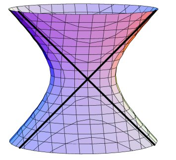
Figure 1: The quadric surface Q
2.3 Special orbits
The 3-dimensional S5 action comes in both real and complex versions. This means that G120 acts on R-the real projective 3-space of points whose coordinates are real numbers that sum to zero. Table 1 in Appendix enumerates some special orbits contained in R while Table 2 describes elements of Q that are fixed by certain members of G120. For ease of expression, I refer to special points (or lines, planes, etc.) in terms of the orbit size: "20-points" (10-lines, 5-planes).
Corresponding to each special point a = (a1,a2,a3,a4,a5) is the plane of points whose coordinates satisfy the equation
|
|
|
Another noteworthy orbit is that of the five coordinate planes consisting of points one of whose coordinates is zero. The intersection of each such coordinate plane with the quadric Q produces a 1-dimensional set-a sphere-with the geometry of the octahedron. Some data for special two-dimensional orbits appear in Table 3.
Finally, a number of special lines appear as intersections of the 5-planes
and 10-planes. Table 4 summarizes the situation.
2.4 Configurations
Some of the geometry that has dynamical significance shows up in various collections of lines. First, the 10-lines whose points have three equal coordinates form a complete graph on the 5-points. Figure illustrates this in two ways. The pentagon-pentagram figure displays a 5-fold symmetry while the double pyramid exhibits the 6-fold symmetry of a single 10-line-represented by the polar axis.
Within each of the icosahedral rulings on Q there are three special line-orbits. These correspond to the 12 vertices, 20 face-centers, and 30 edge-midpoints of the icosahedron. Intersections of lines between rulings give special point structures.
- Two 12-line G60-orbits form six "quadrilaterals" at 24-points.
- Two 20-line G60-orbits form ten quadrilaterals at two pairs of 20-points. (See Figure 3.)
- Two 30-line G60-orbits form 15 quadrilaterals at two pairs of 30-points.
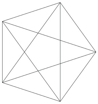
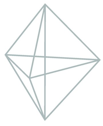
Figure 2: Configuration of 10-lines and 5-points
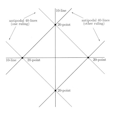
Figure 3: Special configuration of 40-lines and 20-points on Q. At a 20-point there are two 40-lines-one in each ruling on the quadric. This pair of lines corresponds to a pair of antipodal vertices of the dodecahedron. Also shown are the 10-lines determined by a pair of antipodal 20-points.
2.5 Dynamical terminology.
The trajectory of a point x under a map f is the set
of points obtained by applying f iteratively to x. A point
p
is periodic if its trajectory contains p more than once.
A periodic point a in a space X is attracting when the trajectory
of every point near a gets arbitrarily close to a. The basin
of attraction of a is the set of all points attracted to a.
Also, the attractor of f is the set of all attracting points.
2.6 Equivariant maps
The primary tool to be used in solving the general quintic is a map that associates points in CP3 with points in CP3 in a way that respects the action of the group of transformations G120. We want to find a G120-symmetric map (or simply G120-map) with elegant geometry and reliable dynamics; this means that its attractor
- [1)] is a single orbit under G120
- [2)] has a corresponding basin that "fills up" CP3.
2.7 Basic maps
The four maps indicated byf1:(x1,x2,x3,x4,x5)
®
(x1,x2,x3,x4,x5)
f2:(x1,x2,x3,x4,x5)
®
(x12,x22,x32,x42,x52)
f3:(x1,x2,x3,x4,x5)
®
(x13,x23,x33,x43,x53)
f2:(x1,x2,x3,x4,x5)
®
(x14,x24,x34,x44,x54)
are G120-symmetric. Moreover, by combining these with the invariants
|
2.8 Families of symmetric maps
The G120-maps have an algebraic structure relative to the G120-invariants. This means that for an invariant Fl and symmetric map gm of degrees l and m, the product
|
is a symmetric map of degree l+ m. When looking for a map
in a certain degree with special geometric or dynamical properties, my
approach is to express the entire family of symmetric maps for that degree
and, by selecting from a palette of parameters, locate a subfamily and
eventually a single map with interesting behavior.
2.9 Quadric-preserving maps
The rich geometry of the quadric Q provides an intriguing setting
for dynamical exploration. Are there S5-symmetric maps
that send Q to itself? If so, how do they behave on and off Q?
I will describe two species of such maps: one associated with the icosahedron
and the other with the octahedron.
Maps that preserve icosahedral rulings
Were a G120-map to preserve the rulings on Q, its restriction to either ruling would express itself in terms of the basic maps that are symmetric with respect to the one-dimensional icosahedral action-that is, the rotational symmetries of the icosahedron. Maps of this kind occur in degrees 11, 19, and 29. [4] Consequently, the family of 11-maps (maps having degree 11) comes under scrutiny; this family has a palette of 20 parameters.
Choosing parameters to satisfy the demands of the 1-dimensional 11-map with icosahedral symmetry, we obtain a family of ruling-preserving maps.
Restricted to a ruling, the dynamics of each g11 is well-understood.
The 20-lines (under G120) are exchanged in pairs. (Recall
that 20-lines in Q correspond to dodecahedral vertices in the respective
rulings.) Moreover, almost every line in the ruling belongs to the basin
of one of the ten antipodal pairs of the superattracting set of 20-lines.
(See Figure 6 in Appendix.) Thus, for nearly every
point x on Q, there is an "antipodal" pair of intersections
between 20-lines in different rulings which the trajectory of x
approaches.
An octahedral map
Since the orbit of the five coordinate planes has fundamental geometric significance, a map that preserves these sets might exhibit interesting dynamics. Arranging for this requires four of the twenty parameters of the family f11.
The intersection of a 5-plane and the quadric Q is a conic (sphere) with the S4 symmetry of the octahedron. One of the special maps for the octahedral action on CP1 is a degree-5 map that attracts almost every point to the eight face-centers- vertices of the dual cube. Geometrically, the map stretches each face F of the cube symmetrically over the five faces complementary to the face opposite F. As a face stretches, it makes a half-turn so that the vertices and edges land on their antipodes. (See Figure 6 in Appendix.) Under G120, antipodal pairs of octahedral face-centers are pairs of 20-points.
The idea is to find a reliable map that sends Q to itself and behaves like the special 5-map on each of the octahedral conics. Such a map would attract points on Q to the 20-points. We also want the 20-points to be attracting off Q. In degree five there are too few parameters for the purpose. However, the 11-maps provide enough freedom to arrange for elegant geometry.
Each of the 10-lines two of whose coordinates are zero contains a pair of antipodal 20-points. A map that
- [1)] preserves these lines,
- [2)] attracts almost every point on the line to the 20-points, and
- [3)] superattracts in the two directions off the line
would act as a "superattracting pipe" to the quadric. Selecting the remaining parameters accordingly reveals a map h11 with these properties.
It happens that h11 also preserves R-the
S5-symmetric
space of points whose coordinates are real numbers-as well as the 2-dimensional
intersections of R with 1) the five coordinate planes and 2) the
ten planes whose points have two equal coordinates. In the first case there
are four intersections of the 2-dimensional space with the superattracting
10-lines while in the second there is a single such intersection. Each
intersection is a real projective line as well as an "equatorial slice"
of the associated complex projective line-a sphere. When restricted to
such a slice, h11 acts chaotically, meaning that the
trajectory of most of the circle's points gets arbitrarily close to every
point on the circle. A basin portrait for the 5-plane reveals no basins
other than those of the four chaotically attracting 10-lines. (See Figure
8.) The dynamics on the "real part" of the 10-plane shows, in addition
to the chaotic line-attractor, three additional basins at 30-points. (See
Figure 8.)
2.10 A special map in degree six
In the configuration of 10-lines each 5-point lies at the intersection of four lines. (See Section 2.4.) Moreover, these are the only intersections of 10-lines. To take advantage of this structure, a map could have superattracting pipes along the 10-lines and, thereby, have 3-dimensional basins of attraction at the 5-points.
The family of 6-maps has six free parameters. I takes four parameters to obtain maps for which the 10-lines are superattracting in the "off-line" directions. For the remaining two, we get a map f6 whose restriction to a 10-line has the simple form
|
when expressed so that the pair of 5-points on the respective 10-line are 0 and ¥. Recalling that a 10-line is a sphere, such a map attracts all points in the northern hemisphere to the 5-point at ¥ (the north pole) and attracts all points in the southern hemisphere to the 5-point at 0 (the south pole). The equatorial circle-a real projective line-maps to itself chaotically.
Of necessity, f6 preserves each S3-symmetric 10-plane L whose points have two equal coordinates. Furthermore, f6 preserves R-the S5-symmetric RP3. We can get a picture of the map's restricted dynamics by plotting basins of attraction on the intersection of L and R. (See Figures 9 and 10 in Appendix.) The plot shows attraction to three 5-points and one 10-point. However, the 10-point lies on the "equator" of a 10-line. Here, f6 repels in the off-plane direction. Thus, the basin of a 10-point is 2-dimensional. No other attracting sets appear.
A 15-line contains one 5-point, one 15-point, and two 10-points. When restricted to such line, these three points are attracting. (Figure 11 displays portraits.)
Finally, f6 preserves a certain 3-dimensional real projective space that is associated with the group of transformations that fix a 5-point. This RP3 intersects two 10-planes in a space which you can think of as a sphere; this sphere has the symmetry of a double rectangular pyramid. In addition to the 5-point this RP2 contains three 10-points as well as the RP1 through two of the 10-points. Since this line is an equatorial slice through a 10-line where the map looks like
|
3 The sextic-A6 acts in two dimensions
3.1 Basics of A6 and Valentiner's group
Inside the alternating group A6 are twelve versions of the alternating group A5. These twelve subgroups decompose into two systems of six:
- [1)] the permutations that leave one thing unmoved
- [2)] the permutations of the six pairs of antipodal icosahedral vertices resulting from the icosahedron's rotational symmetries.
We can apply the elements of the group A6 to these A5 subgroups. Doing so permutes each of the two systems individually. If we use only the members of one of the A5 subgroups, that subgroup remains unchanged as a whole. As for the five companion subgroups in its system, they move according to the way the icosahedron's rotational symmetries act on the five cubes circumscribed by the icosahedron. Meanwhile, the other system of six A5 subgroups undergo the permutations of the six pairs of antipodal vertices. As a consequence, the intersection of two A5 subgroups in the same system has the same structure as the group A4-the tetrahedral rotations-while two in different systems specify the dihedral group D5-the rotational symmetries of a double pentagonal pyramid.
In the late nineteenth century, Valentiner discovered a group-call it
V-of
360 transformations of 2-dimensional complex projective space that has
the same structure as the group of permutations A6. To
solve the sextic equation, we must find a map on CP2
that is symmetric with respect to V.
3.2 Valentiner geometry
Icosahedral conics
The A5 subgroups of A6 correspond to subgroups of V. Each of the A5 subgroups preserves a respective 1-dimensional conic-a sphere-which thereby has the geometry of the icosahedron. The group V permutes these two sets of six icosahedra in the same way as A6 permutes its two systems of A5 subgroups.
Special orbits
Some of the special icosahedral points on a conic occur at its intersections with the other 11 conics. There are two cases.
- Two conics in the same system intersect in four points; this gives the 20 icosahedral face-centers on a given conic. The overall result is a 60 point V-orbit for each system of conics.
- Two conics in different systems intersect in two points. This gives six pairs of antipodal icosahedral vertices on each conic. These total to a V-orbit consisting of 72 = 6·12 points. Figure illustrates the situation.
As for other special orbits, each of the 45 transpositions in A6 corresponds to a transformation T in V that fixes every point on a line associated with T. In addition, T fixes a point that is not on its associated line. These give V-orbits of 45 lines and 45 points. An V-map typically preserves each of these lines and points; however, as we will see (Section 3.4), something quite different can occur. The typical points on a 45-line provide V-orbits of size 180. Other special orbits occur at the intersections of the 45-lines:
- 36-points on five of the 45-lines
- 45-points on four of the 45-lines
- 60-points on three of the 45-lines (also the face-centers of the icosahedral conics).
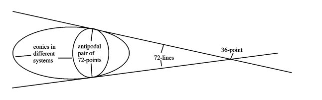
Figure 4: The triangle of one 36-point and two 72-points.
An additional symmetry
The one-dimensional icosahedral group I60 acts on two sets of five tetrahedra each of which corresponds to a quadruple of face-centers on the icosahedron. However, no element of the group sends the tetrahedra of one set to those of the other. Such an exchange occurs by means of orientation-reversing transformations. Some of these are reflections through the 15 great circles of reflective icosahedral symmetry; the remaining 45 are the compositions of odd numbers of these 15 basic reflections-for example, the map that sends a point to its antipode. Extending the orientation-preserving group I60 by such an orientation-reversing transformation produces the group of all 120 symmetries of the icosahedron.
The two systems of conics are the Valentiner analogues of the two sets of tetrahedra. There are orientation-reversing transformations of CP2 that exchange the systems of conics. By taking all combinations of such a transformation with the elements in the group V, we get a new group consisting of 720 symmetries of the Valentiner structure. In analogy to the 15 great circle reflections that produce all 120 symmetries of the icosahedron, there are 36 orientation-reversing transformations that combine to make the 720 Valentiner symmetries. Each of these 36 transformations fixes every point of an associated real-projective plane. (Figure 5 illustrates a geometric construction for these planes.) These 36 planes stand in analogy to the 15 great circles-real projective lines-of icosahedral reflections. A map that respects all 720 of the Valentiner symmetries must send each of these planes to itself. This circumstance allows us to make pictures of such a map's dynamical behavior.
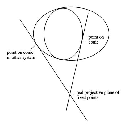
Figure 5: A geometric interpretation of transformations that exchange conics in different systems-indicated by the pair of points.
3.3 Invariant polynomials and symmetric maps
Given a polynomial that is unchanged by the Valentiner group, we express it as a combination of four basic invariants. We can obtain any V-map
from combining these invariants and their derivatives (in the sense of calculus). Again, the idea is to employ a palette of parameters in designing a geometrically elegant map.
3.4 The lowest degree V-map: a case of inelegant dynamics
In degree 16 we find the map of least degree with Valentiner symmetry. This map has the property that it smashes a 45-line down to its associated 45-point. Furthermore, it "blows-up" a 45-point to its companion 45-line. This means that the map spreads a region near the 45-point over the 45-line. The basin portrait (Figure 13) fails to reveal the geometric elegance that we seek.
3.5 A special icosahedral map
Associated with the icosahedron is a degree-19 map that takes each of the 20 faces and stretches it around the icosahedron omitting the opposite face. When iterated, this map attracts almost any point of the icosahedron to one of the six pairs of antipodal vertices. (See Figure 14.)
In the higher dimensional case of the Valentiner group, there is a 19-map h19 that sends each of the 12 icosahedral conics to itself. This means that when we restrict our attention to only one conic, h19 is the map described above. So, we understand much about its dynamics there. Recall that the vertices of the icosahedral conics make up the 72 point V-orbit. It happens that in the direction away from the conic, these points are also attracting.
Moreover, h19 has the additional symmetries of the transformations that exchange the systems of conics. Therefore, it preserves each of the 36 real projective planes associated with these transformations. These spaces look very much like familiar two-dimensional planes. A portrait of the map's dynamical behavior on such a plane appears in Figures 19 through 17.
3.6 A special dodecahedral map
There is another map that preserves conics, though this one is different in kind from that of the 19-map. In this case, we use complex conjugation: an operation on the complex numbers that reflects a point through the axis of real numbers in the so-called plane of complex numbers. This is the sort of orientation-reversing process that exchanges the two sets of five tetrahedra in the icosahedron. We can also apply it to the coordinates of points in 2-dimensional space; this type of operation exchanges the two systems of conics.For each system of conics, but not for both, there is an orientation-reversing map that preserves the six conics individually. When restricted to one of the conics, the map's geometry is to stretch each dodecahedral face onto its complement-the sphere minus the face-while fixing the vertices and edges and sending the face-center to its antipode. You can imagine pushing the face inside the dodecahedron spreading it out symmetrically onto the other 11 faces. This defines an 11-map expressed in complex conjugated coordinates. When iterated, the 12 fixed-points at the vertices attract almost all points on the sphere. Since two conics in one system intersect transversely at the vertices (60-points), these points are attracting in all directions. I plan to study this map and, in a future paper, give a detailed description of its behavior.
A Special orbit data
For ease of reference, the following tables provide descriptions of the special G120 orbits associated with the maps discussed in the text.|
|
|
|
|
|
|
|
|
|
|
|
|
|
|
|
|
|
|
|
|
|
|
|
|
|
|
(0,0,1,w3,w32)
(0,0,1,w32,w3) |
antipodal pair of eight octahedral face-centers on intersections of
Q
and
a coordinate plane ({x1 = 0}, etc.)
w3 = e2 p i/3 |
|
|
(0,1,i,-1,-i)
(0,1,-i,-1,i) |
antipodal pair of six octahedral vertices on intersections of Q and a coordinate plane ({x1 = 0}, etc.) |
|
|
(0,1,1,g,g-) |
antipodal pair of 12octahedral edge-midpoints on intersections of Q
and a coordinate plane ({x1 = 0}, etc.)
g = -1 + Ö2 i |
|
|
|
|
|
|
|
|
|
|
|
|
|
|
|
|
|
|
|
|
|
|
|
|
|
|
|
|
|
|
|
|
|
|
B Gallery of basin portraits
The basin plots that follow are productions of the program
Dynamics
and Dynamics 2 that ran respectively on a Silicon Graphics Indigo-2
and a Dell Dimension XPS with a Pentium II processor. Its BA and BAS routines
produced the images. (See the manuals [5] and [6].)
Each procedure divides the screen into a grid of cells and then colors
each cell according to which attracting point its trajectory approaches.
If it finds no such attractor after 60 iterations, the cell is black. The
BA algorithm finds the attractor whereas BAS requires the user to specify
a candidate attracting set of points. Each portrait exhibits the highest
resolution available-a 720 ×720 grid.
Maps with S5 symmetry
Each of the ten pairs of antipodal dodecahedral vertices-black dots-is a period-2 superattractor. Their basins fill up the sphere. (Bear in mind that points in the space of this plot correspond to lines in either ruling on the quadric surface Q.)
This plot indicates the behavior of h11 restricted to an S4-symmetric conic-the intersection of a coordinate plane and the quadric Q. The four pairs of antipodal vertices of the cube are period-2 superattracting 20-points whose basins fill up the conic.
These show the behavior of the octahedral map h11 on a 15-line and a 30-line respectively.
In the former case, the superattracting points at 0 and ¥ are a pair of 30-points on Q that h11 exchanges. A pair of fixed 10-points accounts for the remaining two basins. At each of these attracting points, the map repels in at least one direction away from the line.
On the 30-line, the superattracting points at 0 and ¥ are a pair of 60-points (antipodal edge-midpoints) on an octahedral conic; the map exchanges the two points. The remaining two basins belong to a pair of 20-points on R. As before, the map repels in at least one direction away from the line at each of these attracting points.
We see the restriction of h11 to a plane with S4 symmetry. The attractor consists of the four lines formed by intersections of R, a coordinate plane, and four of the 10-lines with two zero coordinates. The six intersections of these 10-lines occur at 10-points with three zero coordinates. (See Table 4.) In the picture, two of these intersections occur on the line at infinity. The pictured "lines" are the images of small circles centered along the edges of the inner square. This graphical technique specifically exploits the chaotic and attracting behavior of h11 along each line.
Here, h11 is restricted to a plane with S3 symmetry. The attracting line is the intersection of R, a 10-plane with two zero coordinates and the 10-line at infinity-the light gray basin. The three "attracting" 30-points-they are blowing up-are the vertices of an equilateral triangle.
We see the restriction to the plane determined by the intersection of R and a 10-plane with two equal coordinates. Since this plane is S3-symmetric, we select the coordinates so that the three 5-points are vertices of an equilateral triangle that is symmetrical about the center. Three of the superattracting pipes contain this triangle.
The map sends the indicated circle to the ``triangle" shown here. This triangle strongly aligns itself with the superattracting pipes through the 5-points. The attractor at the center is a 10-point. In the direction away from the plane, f6 repels at this site along a superattracting pipe. The three "spokes" at basin boundaries are pieces of 15-lines each of which passes through a secondary basin that contains a point that maps to the central 10-point.
This shows f6's critical set-where the map folds the plane over-superimposed on the basin portrait. The critical contour is a Mathematica plot. The curve crosses itself at the 5-points. All but six critical points appear to belong to the basin of either a 5-point or the central 10-point. The six exceptions lie on the 15-lines at basin boundaries. If this is so, then there is no other attracting site.
We see f6 restricted to a 15-line that maps to itself. The coordinates place the single 5-point at the center and the two fixed superattracting 10-points at symmetrical locations on each side. At the latter points, the map repels in all directions off the line.
This approximately shows the boxed region of the previous plot.
The space here is the plane where an S4-invariant RP3 and a 10-plane intersect. The intersection of the plane and the associated 10-line with three equal coordinates is the central vertical axis. By plotting the trajectory of one of its generic points, this line reveals itself as a chaotic attractor; the plot shows roughly 20,000 iterates. The map also attracts at a 5-point and 10-point.
Figure 6: Platonic dynamics
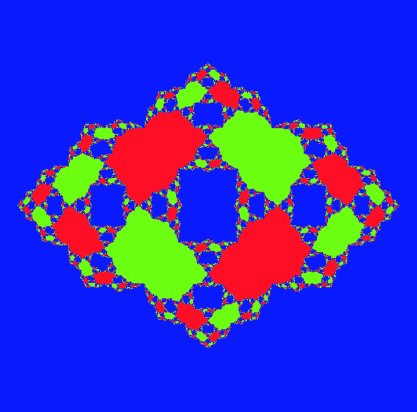
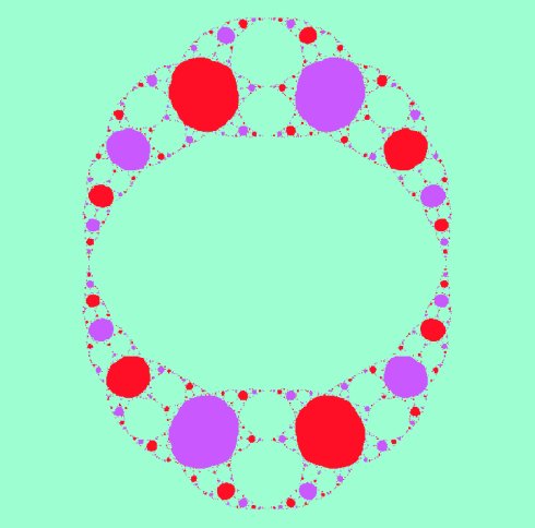
Figure 7: Three basins of attraction for h11restricted to a 15-line (left) and a 30-line (right)
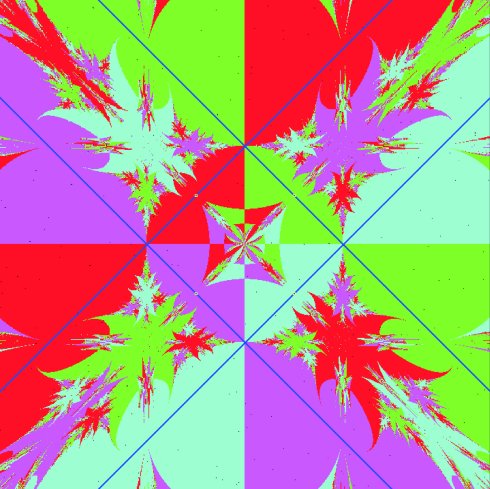
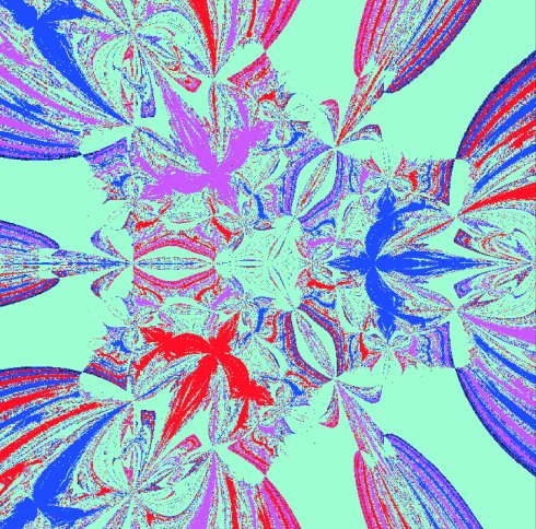
Figure 8: Chaotic attractors for h11 on a plane with S4 symmetry (left) and a plane with S3 symmetry (right)
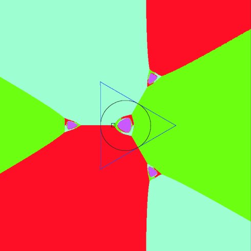
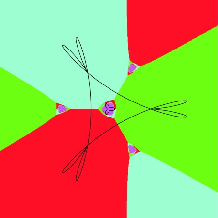
Figure 9: Four basins of attraction for f6 restricted to an plane
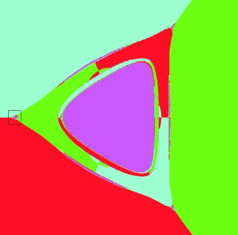
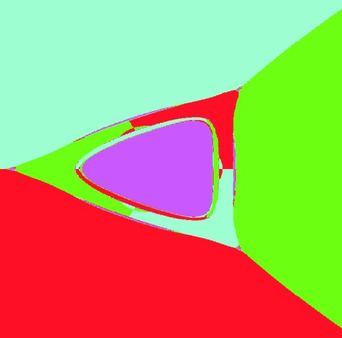
Figure 10: Detail of the left cusp of central basins in Figure 9
Figure 11: Three basins of attraction for f6 restricted to a 15-line (left) and magnified view of the boxed region (right)
Figure 12: Chaotic attractor for f6 on a plane
Maps with A6 symmetry
When "restricted" to a 45-line, the degree-16 map "mostly" converges to one of the 45-points on the line. Does this occur for almost every point on the line? Do the black specks consist of points whose trajectories fail to converge to one of the four attracting 45-points that lie in the large central basins? The BAS algorithm checked 60 iterates before concluding that a trajectory did not converge.
The degree-19 map with icosahedral symmetry attracts almost all points in the sphere to an antipodal pair of vertices. Each of the six colors corresponds to such a pair and the three large basins each contain a vertex. For the conic-preserving h19, the basin plot on each conic looks like this one. Moreover, each basin is the 1-dimensional intersection of a 2-dimensional basin.
The image shows the behavior of h19 on one of the 36 real projective planes determined by the basic conic-exchanging transformations. Each large radial basin contains one of the 72-points and come in pairs as do the period-2 attractors. Notice the repelling behavior along the 45-lines and particularly at their intersection in the 36-point at the center.
Shown here are trajectories, colored according to their destinations, of the points in the vertical strip on the left. Many of the points in the strip map inside the hazy pentagon whose vertices lie on the 45-lines-the inner "star" is nearly filled. Circumscribing this pentagon is the outer star-like piece of the critical set shown in Figure 16. Furthermore, the pentagon seems to be the image of the inner pentagonal oval. Accordingly, the map folds the plane along the pentagon's edges just outside of which the 72-points make their presence seen in the dense streaks. Compare this pattern of streaks to that of the 72-lines shown in Figure 16. Figure 17 illustrates this local "squeezing" at a 72-point.
The lines tangent to a conic at the 72-points form an orbit of 72 lines. For any one of the 36 planes of reflection associated with transformations that exchange the systems of conics-call such a plane R, there are five pairs of the 72-lines that intersect R in lines. The picture shows their configuration in the plane of Figure 15. Each pair receives a single color according to the scheme of the basin plot. A given pair of lines passes through the associated pair of 72-points; they intersect in the corresponding fixed and repelling 36-point.
Here is a Mathematica contour plot on R of the set of points in R that satisfy the equation F6 = 0. This curve is the critical set of h19-where folding over takes place. The superattracting 72-points are the inflection points.
The green horizontal line corresponds to the intersection of the reflection plane R and the 36-line passing through the pair of green 72-points from the basin plot. The dark curve is where h19 sends the line. Sitting at the sharp cusps are the 72-points which the map exchanges. As indicated in the caption to Figure , the line folds over at these critical points. The upper two sharp turns correspond to where the line passes through the yellow and red "streaks" that approximate 72-lines.
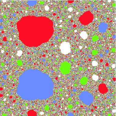
Figure 13: Dynamics of the 16-map
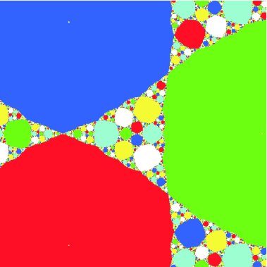
Figure 14: Icosahedral dynamics of the 19-map
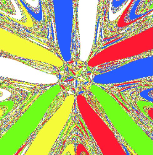
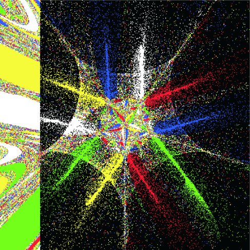
Figure 15: Dynamics of h19 on a plane with 10-fold symmetry
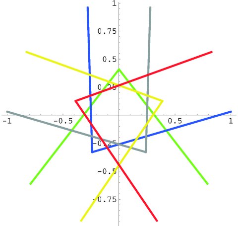
Figure 16: Configuration of 72-lines and critical set of h19
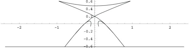
Figure 17: Image of a 36-line under h19
References
- [1]
- S. Crass. Solving the sextic by iteration: A study in complex geometry and dynamics. Experiment. Math. 8 (1999) No. 3, 209-240.
- [2]
- S. Crass, 2000. Solving the quintic by iteration in three dimensions." To appear in Experiment. Math. 10 (2001) No.1, 1-24.
- [3]
- Mathematica notebook and data files that implement the quintic- and sextic-solving algorithm based on the dynamics of f6. See http://www.csulb.edu/ ~ scrass.
- [4]
- P. Doyle and C. McMullen. Solving the quintic by iteration. Acta Math. 163 (1989), 151-180.
- [5]
- H. Nusse and J. Yorke. Dynamics: Numerical Explorations Springer-Verlag, 1994. UNIX implementation by E. Kostelich.
- [6]
- H. Nusse and J. Yorke. Dynamics: Numerical Explorations, 2e Springer-Verlag, 1998. Computer program Dynamics 2 by B. Hunt and E. Kostelich.