|
Gwen Fisher Mathematics Department California Polytechnic State University San Luis Obispo, CA 93407 Blake Mellor Mathematics Department Loyola Marymount University Los Angeles, CA 90045-2659 Abstract
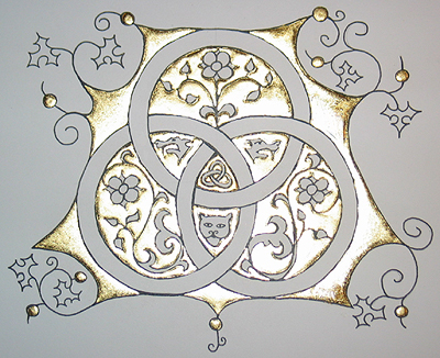
1. Introduction There is a long tradition of abstract geometric designs in the art of the Celtic peoples of ancient Britain, Scotland and Ireland, including spirals, key patterns and, in the Christian era, knots and interlacings [1]. Complex knotwork patterns were used profusely in the Celtic illuminated manuscripts, such as in the Books of Durrow (early 5th to early 6th century), Kells (middle 6th to early 8th century), Lindesfarne (late 7th century), and Grimbald of St. Bertin (early 11th century). In these manuscripts, interlacing designs (both purely geometric, as in Figure 1, and incorporating animal figures) fill areas and are used as borders for text and illustrations. Françoise Henry called these designs a "sacred riddle" [7], and their symbolic meaning is a fascinating and unresolved issue in Celtic art history. James Trilling [10] has theorized that knotwork designs were, like the crosses that they commonly accompanied, protections against evil: the complex designs would trap and confuse the "evil eye".
Figure 1: A knotwork design, from [5] Whatever their meaning, the complexity of Celtic knotwork designs is evidence of substantial mathematical sophistication [4], and their design and analysis lead to many mathematical questions. Several authors [2, 9] have studied methods by which the Celtic artists may have constructed their designs. Peter Cromwell [3] studied the symmetries of Celtic knotwork as strip patterns. In this paper we look at a deceptively simple question: How many different components (closed loops) are there in a given knotwork design? This is the first step towards measuring the "complexity" of a design, and perhaps (if Trilling is correct) its protective powers. It is also a question particularly appropriate for Celtic art. While knotwork and interlacing designs appear in many traditions, the designs are not always "closed off" into a finite number of loops. In Islamic art, for example, interlace patterns are often part of an infinite plane, in which some strands never close into loops at all [6]. In addition to assisting in the analysis of Celtic art, methods for determining the number of components in a design can assist artists in creating new work. Some writers have claimed that the ancient Celts used designs with a single component to represent continuity and eternity (though there seems to be no clear evidence one way or the other) [9]. Modern artists may do the same or, conversely, prefer more than one component so that the design may be colored with multiple colors. We will not give a complete answer to the problem of counting
components. Celtic knotwork designs can easily become immensely complex
the design in Figure 1 is a relatively simple example,
yet its structure still exceeds our methods of analysis and it will take
much more work to develop a general approach. We will only examine a few
fundamental designs: the basic knotwork panels and their extensions to
rectangular and circular border designs. Our method is to study how the
braiding in the designs changes the order of the strands, so each design
corresponds to some permutation of the strands. With this viewpoint, to
compute the number of components in the design, we count the number of
cycles in the permutation, which is a relatively easy mathematical problem.
Along with the details of our results we will provide several examples
and illustrations.
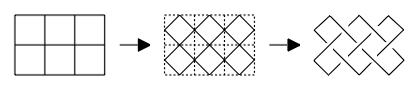
2. Counting Components in Knotwork Designs 2.1 Knotwork Panels. The history of the development of Celtic knotwork designs is still a subject of debate. One popular theory, proposed by J. Romilly Allen [1], is that Celtic knotwork (as well as other interlace traditions) developed from plaitwork panels used in Roman decoration. The basic plaitwork panel can be described using a square grid with p rows and q columns. The process is illustrated in Figure 2. We begin with the grid, and in each square draw the inscribed square whose vertices are the midpoints of the original square. Where two of the inscribed "diamonds" meet, we insert a crossing: if the diamonds are meeting on a vertical line of the original grid, the strand connecting the bottom left to the top right will be on top; if they are meeting on a horizontal line, the strand connecting the top left to the bottom right will be on top. Finally, we erase the original square grid. (We could, of course, reverse all the crossings; but this would not affect the number of components in the design.) To get the traditional "ribbon" designs, as in Figure 3, we simply thicken the knot into a ribbon.
Figure 2: Constructing a basic 2 ´ 3 knotwork panel More complicated knotwork designs are formed from the basic plaitwork panel by making breaks in the pattern erasing a crossing and rejoining the four strands in one of the other two possible ways (top to top and bottom to bottom, or right to right and left to left). This leads to designs such as Figure 1. However, in this paper we will only be considering the basic plaitwork pattern as we will see, even this is not a trivial problem! The construction that we have given of the plaitwork pattern
is more convenient for the mathematician than for the artist for a practical
method for creating these panels (and many other designs) see Bain [2]
and Meehan [9]. Notice that these knots and links are
alternating
- as we travel along one strand, the crossings alternate between over-
and under-crossings. A component of a design is a closed loop in
the design. If the design has only one component, we will call it a knot;
otherwise, we will call it a link. Our first problem is to count
the number of components in the basic panel design. It is well known that
a p ´q panel will have one component
when
p and q have no common factors, and that a p´p
square panel has p components [2, 3].
We will generalize these facts to give a formula for the number of components
in any panel. We will prove our formula in two ways one that is
more intuitive, and one that introduces the mathematical machinery of permutations
that we will use in the rest of the paper.
Figure 3: Examples of knotwork panels Theorem 1: The number of components in a p´q knotwork panel is given by the greatest common divisor gcd(p, q). Figure 3 shows two examples of Theorem
1. In particular, the 4 ´ 6 panel
has 2 = gcd(4, 6) strands, and the 12 ´
15 panel has 3 = gcd(12, 15) strands. We will first approach this result
from an intuitive, topological point of view. Since our construction of
the knotwork panel begins with a square grid, every line in the design
has slope 1 or -1. Imagine an ant traveling along one strand in the panel,
beginning at the left side of the panel. Eventually the ant will traverse
the entire component and begin to retrace its steps how long will this
take? Since the strands only change direction at the boundaries of the
grid, to return to its starting point (facing in the same direction that
it started) the ant will need to follow the strand across the grid and
back some number of times both horizontally and vertically. So the
ant will travel a distance 2pj vertically and a distance 2qk
horizontally
(for some integers j and k). (The factor of 2 is needed because
the ant travels across the grid and back.) Since the ant is always traveling
one unit vertically for each unit horizontally (and vice-versa), this means
that 2pj = 2qk, where j and k are integers.
For each complete circuit of the component,
j (or k) represents
the number of times the ant travels across the panel and back in the vertical
(or horizontal) direction, respectively. Our goal is to find the smallest
values of j and k for which this occurs (to find the first
time the ant returns to its starting point). This means that pj = qk
= lcm(p, q), where lcm(p, q) is the least
common multiple of p and q. Since pq = lcm(p,
q)·gcd(p,
q),
we can conclude that Since k is the number of times the ant walked across
the full width of the panel in the horizontal direction, it also gives
the number of times the ant turned around at the left side of the panel.
This number did not depend upon which strand the ant started, so every
strand must meet the left side the same number of times. Since the total
number of times all strands meet the left side of the panel is p,
the number of different strands is A nice consequence of this argument is that, since each
component of the design meets the left (and right) side of the panel While this approach to the problem is very natural, it
is difficult to extend it to other designs. We will describe another approach,
based on the mathematics of permutations, which extends very nicely to
several other designs. To begin with, imagine a vertical strip of a panel.
A p ´ q panel has 2p
strings running horizontally across it, intertwining with each other (several
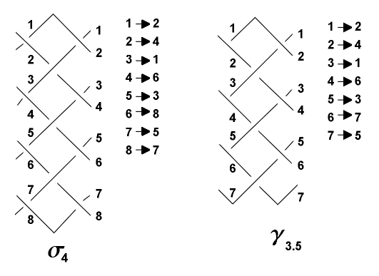
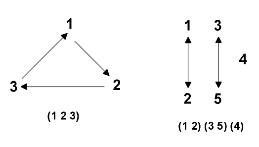
Figure 4: Permutations of strings. Permutations are often represented using cycle notation.
For example, the permutation of the set {1, 2, 3} that sends 1 to 2, 2
to 3 and 3 to 1 is represented by the 3-cycle (123). The permutation of
the set {1, 2, 3, 4, 5} which sends 1 to 2 and 2 to 1, 3 to 5 and 5 to
3 and leaves 4 fixed would be written (12)(35)(4). We can visualize these
cycles as shown in Figure 5.
Figure 5: Cycles in permutations We can "multiply" permutations by performing one after the other and looking at the result. Products of permutations are traditionally read from right to left. For example, the product (123)(12)(35)(4) of the permutations in Figure 5 sends 1 to 2, and then 2 to 3, so the product sends 1 to 3. Similarly, we can see that the product sends 3 to 5, and 5 to 1, so we have a cycle (135). Finally, the product fixes 2 and 4. In cycle notation, we write that (123)(12)(35)(4) = (135)(2)(4). Returning to our knotwork panel: In cycle notation, the permutation s4 in Figure 4 is (12468753). In general, the permutation is sp = (124...2p 2p-1 2p-3...53), which is always a 2p-cycle. When the strings hit the left or right sides of the panel, they "bounce" with a permutation dp = (12)(34)(56)...(2p-1 2p) because neighboring strings switch places. So if we follow the strings from the left side of the
panel to the right and back again, bouncing off each end, when we return
to our original position (moving once again to the right), the total permutation
is given by the product First note that In the following sections, we will extend this approach to several other basic designs. 2.2 Circular Borders. Circular motifs are also
common in Celtic knotwork designs, often appearing as elements in larger
designs, such as stone carvings or illuminated manuscripts [2,
8].
They are also found in modern designs influenced by the Celtic tradition.
Figure 6: The 2.5 ´
12 circular border has 1 component and the 2 ´
12 circular border has
The simplest circular knotwork design is made by bending a p ´ q knotwork panel into a circle, and joining the left and right sides to get a p ´q circular border. Three such designs are shown in Figure 6. Cromwell [3] noted that knotwork panels must have an even number of horizontal strings in order to close up (a p ´q panel has 2p strings). In circular designs, however, there can be an odd number of strings, so p can be a half-integer as well as an integer. Figure 6 shows examples of each type. There is, once again, a simple formula for the number of components in the design. The simplest circular borders are well known to knot theorists, although by other names the 1 ´ 3 circular border is the trefoil knot, and the 1.5 ´ 3 circular border is the Borromean link. Figure 6 shows the Borromean link; a tiny trefoil knot can be seen in the center of the design. Theorem 2: The number of components in a p´ q circular border is gcd(2p, q). Notice that when p is a half-integer, 2p
is odd, so the design will have an odd number of components. As an example,
in Figure 6, the figure on the left has gcd(5, 12) =
1 component, the figure in the middle has gcd(4, 12) = 4 components, and
the Borromean link has gcd(3, 3) = 3 components. We will prove Theorem
2 using the permutation technique we developed in Section
2.1. We first consider the case when
p is an integer, so the
permutation across one "diamond" is once again sp.
In the circular case, the permutation of the strings as we travel once
around the design is On the other hand, if p = k + 1/2 for some integer
k,
then we need to consider a slightly different permutation. In this case,
there are 2p = 2k + 1 strings winding around the design.
The permutation of the strings as we move one unit clockwise around the
design (i.e. one "qth" of the way around) is given by gp
= (1 2 4...2p-1 2p 2p-2...5 3), a 2p-cycle.
The right illustration in Figure 4 shows the case when
p
= 3.5. So the permutation as we make a complete circuit of the design is 2.3 Rectangular Borders. Our methods are easily adapted to looking at rectangular borders, or frames of constant width. In general, frames have three parameters: the height p, the breadth q and the width (of the band) n. We will refer to such a frame as a p ´ q frame of width n. Note that n, as for circles, may be either an integer or a half-integer, such as 1.5. Figure 7 shows several examples.
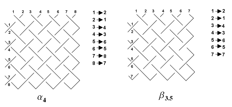
Figure 7: Examples of frames: 5 by 5 of width 2, 5 by 5 of width 1.5, 5 by 6 of width 2, and 5 by 7 of width 2 The number of components in a frame design is given by the following theorem: Theorem 3: The number of components in a p´q frame of width n is equal to 2gcd(|p q|, n) (if n is an integer) or to gcd(|p q|, 2n) (if n is a half-integer k + 1/2, with k an integer). Here we require 2n < min (p, q). Notice that, as with circles, if the width of the frame is an integer then there is an even number of components, and if the width is a half-integer then there is an odd number of components. If we apply this result to the examples in Figure 7, we see that the designs (from left to right) have 2gcd(5 5, 2) = 4 strands (0 is divisible by anything), gcd(5 5, 3) = 3 strands, 2gcd(6 5, 2) = 2 strands and 2gcd(7 5, 2) = 4 strands. Once again, we will use permutations as with the circular borders, the arguments are simpler and more natural than with the panels, since we do not need to worry about "bouncing" off the sides. The permutation of the strings of the design as we go along the sides is given by sn or gn, depending on whether n is an integer or a half-integer. In addition, we need to determine what happens as we "turn a corner" in the design. We will denote the permutation of the strings around a corner by an if n is an integer, and by bn if n is a half-integer. Figure 8 illustrates a4 and b3.5. In general, we can see that an
= (12)(34)(56)...(2n-1 2n); in fact, an
is the same as dn from Section
2.1. Similarly, bn = (12)(34)(56)...(2n-2
2n-1)(2n) (note that in this case 2n is odd). Recall
from Section 2.1 that
Figure 8: Permutation of strings around corners. If n is an integer, the permutation of the strings around the frame is given by the product of the four sides and four corners:
The number of disjoint cycles in this permutation (and hence the number of strands in the design) is therefore gcd(|2(q p)|, 2n) = 2gcd(|p q|, n). If n = k + 1/2, the permutation of the strings around the frame is given by
The number of disjoint cycles is therefore gcd(|2(q p)|, 2n) = gcd(2|q p|, 2k + 1). Since 2k + 1 is odd, the greatest common divisor must be odd, so we can ignore the factor of 2 in the first term. So the number of strands of the design is equal to gcd(|p q|, 2n). 2.4 Half-frames or L shapes. We can apply the techniques we have developed to a wide range of designs involving a strip of constant width that makes right angle turns. A simple example of such a design is half of a frame, or an L shape. A p ´qL of width n has height p, base length q and is made from a strip of width n. As with panels, n must be an integer. Examples of L shapes are shown in Figure 9. Theorem 4: The number of components (strands) in a p ´qL
shape of width n is gcd(|p q|,
n).
Figure 9: Examples of L shapes:4 by 5 of width 2, 5 by 5 of width 2, 6 by 6 of width 2. We can check this formula on the examples in Figure 9.
The design on the left has gcd(5 4, 2) = 1 strand, the design in the
middle has gcd(5 5, 2) = 2 strands, and the design on the right has gcd(6
6, 2) = 2 strands. We prove the formula using the same methods as before.
Using the permutations we have defined in the earlier sections, the permutation
of the strings in the L is obtained by beginning at the top, traveling
to the bottom, turning a corner, traveling to the end, "bouncing" and eventually
returning to our original position (after turning the corner and bouncing
off the top to face down again). This permutation is
So the number of disjoint cycles is gcd(2|p q|, 2n)
= 2gcd(|p q|, n). As with knotwork panels, each
component of the design is counted by two of these cycles, so the number
of components is gcd(|p-q|, n).
3. Conclusion Obviously, there is much more work to be done. Another
common design is the Celtic Cross, and many other designs do not involve
strips of constant width, but have strips of different widths joining with
each other these will require new techniques to analyze. And, of course,
we have not even begun to analyze the effects of "breaking" the basic plaitwork
pattern. We have presented a few basic ideas and results, but these are
only a first step.
References [1] Allen, J.R., Celtic Art in Pagan and Christian Times, Methuen, London, 1904 [2] Bain, G., Celtic Art: The Method of Construction, Dover, New York, 1973 [3] Cromwell, P.R., "Celtic Knotwork: Mathematical Art", Mathematical Intelligencer, Vol. 15, No. 1, 1993, pp. 36-47 [4] Doran, B., "Mathematical Sophistication of the Insular Celts Spirals, Symmetries, and Knots as a Window onto their World View", Proceedings of the Harvard Celtic Colloquium, Vol. 15, 1995, pp. 258-289 [5] Gillman, P., http://www.boulder.net/~gillman/prism/drawing.html [6] Grunbaum, B. and Shephard, G.C., "Interlace Patterns in Islamic and Moorish Art", Leonardo,, Vol. 25, No. 3/4, 1992, pp. 331-339 [7] Henry, F., Irish Art in the Early Christian Period, Cornell University Press, Ithaca N.Y., 1965 [8] Laing, L. and J., Art of the Celts, Thames and Hudson, London, 1992 [9] Meehan, A., Celtic Design: Knotwork, Thames and Hudson, New York, 1991 [10] Trilling, J., "Medieval Interlace Ornament: the Making of a Cross-Cultural Idiom", Arte Medievale, Vol. 9, 1995, pp. 59-86
|