|
Jay Kappraff
Gary W. Adamson
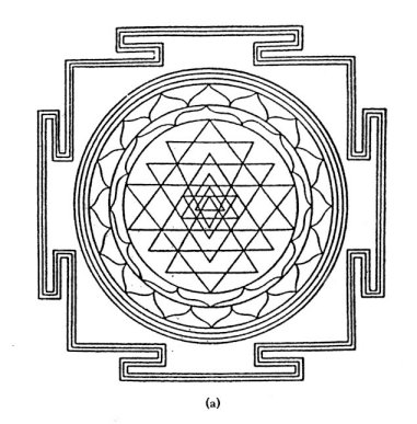
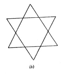
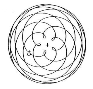
1. Introduction Through many cultures, star polygons were used as sacred symbols with the star of David and the Sri Yantra Hindu patterns shown in Figure 1a and 1b as two examples. The fact that Venus traverses a five-pointed star over an eight-year cycle in the heavens as seen from the Earth, shown in Figure 1c, was known to ancient civilizations. Also the designs of ancient sacred geometry use a small vocabulary of proportions such as Ö 2, Ö 3, the golden mean t = (1+Ö 5)/2 and the silver mean q = 1 + Ö 2. I will show that all of these constants can be related to the edge lengths of star polygons and that they are ultimately related to a sequence of numbers called silver means the first of which is the golden mean. These silver means will also be shown to be generalizations of the imaginary number i in some sense. The geometry of the star heptagon will be found to be particularly interesting. I have previously shown that star polygons are also related to the chaotic dynamics of the logistic equation [Kappraff 2002].
Figure 1
2. Star polygons A regular star polygon is denoted by the symbol {n/k} where n is the number of vertices and edges while k indicates that each vertex is connected to the k-th vertex from it in a clockwise direction. Under certain conditions a regular star polygon can be drawn in a single stroke such as polygon {5/2} in Figure 2a or in more than one stroke as polygon {6/2} in Figure 2b. Is there a simple rule that predicts whether the polygon is irreducible (can be drawn in a single stroke) or reducible (cannot be drawn in a single stroke)? The answer is simple: a polygon {n/k} will be connected if and only if n and k are relatively prime. 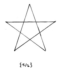 
Figure 2
Only connected stars are considered to be star polygons. For example, {6/2} actually corresponds to the connected 3-gon {3/1}. As a result of the fact that n and k must be relatively prime, there are as many regular n-gons as there are positive integers relatively prime to n denoted by the Euler phi-function f (n). For example, there are f (7) = 6 species of star 7-gons and f (12) = 4 species of 12-gons. The three clockwise oriented 7-gons are shown in Figure 3 with three identical but counterclockwise oriented 7-gons not shown. Of the 12-gons illustrated in Figure 4 only {12/1} and {12/5} are actual 12-gons. They are the two clockwise oriented 12-gons with the two counterclockwise 12-gons not shown. 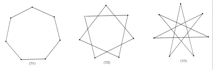
Figure 3
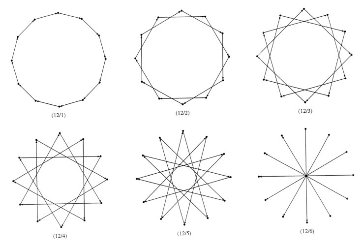
Figure 4
The edges of a star n-gon are the diagonals of the regular n-gon. By determining the lengths of the n–3 diagonals that can be drawn from a given vertex of a regular n-gon, including the edge, we are also determining the lengths of the edges of various species of star n-gons. Furthermore, when all polygons are normalized to radius equal to one, the diagonals and edges of any m-gon reappear in n-gons whenever n is a multiple of m. For example, in Figure 4 the edges of the triangle, square and hexagon appear as diagonals of a regular 12-gon. In this way we are able to determine all of the star m-gons related to an n-gon by considering all of the factors of n. For example, consider the 12-gon. Its factor tree is, 3 ® 6 ® 12 ¬ 4 ¬ 2. (1) The edges of the triangle reappear as diagonals of the hexagon and the 12-gon. Also the edges of the square reappear within the 12-gon. The factor 2 corresponds to the diameter {12/6} in Figure 4 and can be thought of as a polygon with two edges, referred to as a digon {2/1}. In some limiting sense a single vertex can be thought to be a polygon with a single edge of zero length {1/1}. If we add up the total number of star polygons corresponding to these factors we get f (1) + f (2) + f (3) + f (4) + f (6) + f (12) = 12. (2) These are all the star polygons related to the 12-gon. In addition to the single vertex and the digon, five of these have their edges oriented clockwise while five mirror images have retrograde edges. It can be shown that, in general,
where the summation is taken over the integers that divide evenly into n. Star polygons are connected to number theory in many ways. One striking example is due to H.S.M. Coxeter in which the star polygon gives an elegant proof of Wilson’s Theorem. Wilson’s Theorem: For p a prime number, (p–1)! = –1 (mod p) or the integer (p–1)! + 1 is divisible by p. Proof: For any p-gon there are clearly (p–1)! distinct p-gons. Since f (p) = p–1, p–1 of them are regular while the others are irregular. Since the regular polygons are invariant under rotation while the irregular ones are not, each irregular configuration gives a new polygon under rotation about the center through the angle between adjacent vertices. So if there are N classes of irregular polygons, when these are rotated about the p vertices, there are Np irregular polygons. Therefore, (p–1)! = Np + p–1 or (p–1)! + 1 = Np. And, as a result, (p–1)! + 1 is divisible by p
or (p–1)! = –1 (mod p).
3. Pascal’s Law and Star Polygons Consider Pascal’s triangle.
Table 1 Starting from the left in Table 1 the
diagonals: 111…, 123…,136…, etc. appear as columns in which each
successive column is displaced, in a downward direction, from the previous
column by two rows. The rows of Table 2 can be seen to
be the diagonals of Pascal’s triangle related to the Fibonacci sequence
with the sum of the elements of row n being the n-th Fibonacci
number. This table, referred to as the Fibonacci-Pascal Triangle or FPT,
is associated with the coefficients of a series of polynomials, F1(n),
(the superscripts are the exponents of the polynomials) [Adamson 1994].
(n,k) = (n-1,k) + (n-2,k-1) where (n,k) denotes the number in the n-th row and k-th column. For example, (7,3) = (6,3) + (5,2) or 10 = 6 + 4. Also, beginning with 1 and x, each Fibonacci polynomial F1(n) is gotten by multiplying the previous one, F1(n-1) by x and adding it to the one before it F1(n–2), e.g., F1(3) = x F1(2) + F1(1) or x3 + 2x = x(x2 + 1) + x. Letting x = 1 in the polynomials yields the Fibonacci sequence: 1 1 2 3 5 8 ... The ratios of successive numbers in this series converge to the solution to x – 1/x = 1 or the golden mean t which I shall also refer to as the first silver mean of type 1 or SM1(1). Letting x = 2 yields Pell's sequence: 1 2 5 12 29 70 ... (e.g., to get a number from this sequence, double the preceding term and add the one before it). The ratio of successive terms converges to the solution of x – 1/x = 2 or the number q = 1 + Ö 2 = 2.414213..., referred to as the silver mean or more specifically as the 2nd silver mean of type 1, SM1(2). Letting x = 3 yields the sequence: 1 3 10 33 109 ... (e.g., to get a number from the sequence, triple the proceeding term and add the one before it). The ratio of successive terms converges to the solution to x – 1/x = 3 which is the 3rd Silver Mean of type 1 or SM1(3). In general letting x = N, where N is either a positive or negative integer, leads to an approximate geometric sequence for which, xk+1 = Nxk + xk-1 , and whose ratio of successive terms is SM1(N) which satisfies the equation, x – 1/x = N. (3a) When the polynomials in Table 2 have alternating signs they are denoted by F2(x), and upon letting x = N, xk+1 = Nxk – xk-1 , and whose ratio of successive terms is SM2(N), silver means of the second kind, which satisfies the equation, x + 1/x = N. (3b)
4. Lucas Version of Pascal’s Triangle Fibonacci and Lucas sequences are intimately connected. The standard Fibonacci sequence, {Fn}, is: 1 1 2 3 5 8 13 … while the standard Lucas sequence, {Ln}, is 1 3 4 7 11 18... where Ln = Fn-1 + Fn+1. Adamson has discovered another variant of Pascal’s triangle related to the Lucas sequence. In fact this Lucas-Pascal Triangle or LPT demonstrates that silver mean constants and sequences are part of an interrelated whole. Along with the FPT these tables are carriers of all of the significant properties of the silver means. To construct the LPT, create a new "Pascal’s triangle"
with 1’s along one edge and 2’s along the other as shown in Table
3.
Table 3. A Generalized Pascal’s Triangle As before each diagonal becomes a column of the LPT
in which the elements in each successive column are displaced downwards
by two rows. The exponents of the corresponding polynomials are sequenced
as for the FPT. You will notice that the numbers in each row sum
to the Lucas sequence and therefore I refer to the associated polynomials
as Lucas polynomials L1(n) to distinguish these
from Lucas polynomials with alternating signs denoted by L2(x).
Table 4. Lucas-Pascal’s Triangle Beginning with 2 and x, a Lucas polynomial is generated by the recursive formula: L1(n) = x L1(n-1) + L1(n-2), for example L1(3) = xL(2) +L1(1) or x3 + 3x = x(x2 + 2) + x . Setting x = 1,2,3,… in the Lucas polynomials generates
a set of Generalized Lucas sequences that are related to the SM1(N)
constants. Many interesting properties of these sequences are described
in [Kappraff 2002]. They also lead directly to an
infinite set of generalized Mandelbrot sets [Kappraff
2002].
5. The relationship between Fibonacci and
We have discovered a simple relationship between the roots of both the Fibonacci and Lucas polynomials with alternating signs and the diagonals of regular polygons when the radii of the polygons are taken to be 1 unit. For odd n, the positive roots of the n-th Lucas polynomial, L2(n), with alternating signs equal the distinct diagonal lengths dk for k>1 and edge d1 of the n-gon of radius 1 unit where dk = 2sin kp/n for k = 1,2,…, (n–1)/2 (4) where the labeling of the n–1 diagonals is illustrated in Figure 5. 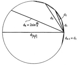
Figure 5
Example 1: For a pentagon, d1 and d2 = td1 where d1 = (Ö (1+ t2))/t are the roots of L2 (5): x5 – 5x3 + 5x = 0, This gives the familiar result that the ratio of the diagonal to the edge of a regular pentagon is the golden mean t . Example 2: For a heptagon, d1, d2 = rd1 and d3 = sd1 where d1 = Ö [(rs –1)/rs ] are the roots of L(7) where r = 1.8019377… and s = 2.2469796… : x7 – 7x5 + 14x3 – 7x = 0, The numbers have additive properties much as the golden mean and this will be discussed in the next section. For even n, the positive roots of the (n–1)st Fibonacci polynomial with alternating signs F2(n–1), equal the lengths dk of the distinct diagonals of regular n-gons of radius 1 unit where dk = 2sinkp/n for k = 1,2,…, (n–2)/2. (5) For polygons with even n, one of the diagonals is twice the radius or 2. This diagonal is not one of the roots. Example 3: For a hexagon, d1 and d2 = Ö 3d1 where d1 =1 are the roots of F(5): x5 – 4x3 + 3x = 0. Example 4: For an octagon, d1, d2 = Ö (qÖ 2)d1 and d3 = qd1 where d1 = Ö (Ö 2/q ) are the roots of F(7) : x7 – 6x5 + 10x3 –4x = 0. The results for several polygons are summarized in Table 5. The diagonals are normalized to an edge value of 1 unit by dividing by d1. 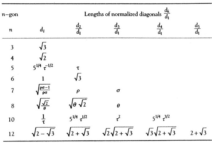
Table 5. Lengths of Normalized Diagonals of n-gons We find the curious property that both the sum and product of the squares of the diagonals of an n-gon (including the edge) equals an integer and that this integer equals n for odd values of n. For example, d12 + d22= 5 and d12d22 = 5 for the pentagon, while, d12 + d22 + d32 = 7 and d12d22d32= 7 for the heptagon. Not only are the diagonals of regular polygons determined by Equations 4 and 5, but the areas A of the regular n-gons with unit radii are computed from the elegant formula,
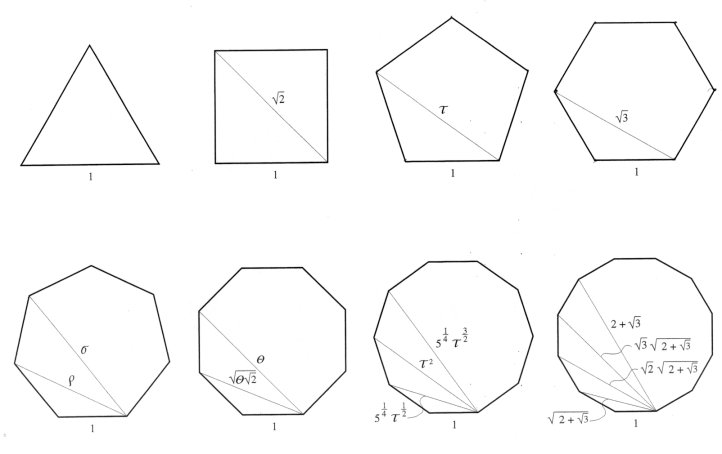
From this equation the square is found to have area 2 units while the 12-gon has area 3 units. It can also be determined that if n approaches infinity, then A approaches p , the area of a unit circle. Notice that the key numbers in the systems of proportions based on various polygons present themselves in Table 5: t–pentagonal system; q and Ö 2 –octagonal; Ö 3, 1+ Ö 3, and 2+Ö 3 –dodecahedral; r and s –heptagonal, and these are pictured in Figure 6. Figure 6
6. The Relationship between Number and the Geometry of Polygons Since the unique diagonals of an n-gon correspond to the roots of a polynomial, the fact that these diagonals recur in any m-gon where n is a multiple of m serves to factor the polynomial into polynomials of smaller degree with integer coefficients. For example, the polynomial F2(9) of the 10-gon factors into the product of L2(5) of the 5-gon and F2(4), i.e., F2(9) = L2(5)×F2(4) or, x9 – 8x7 + 21x5 – 20x3 + 5x = (x4 – 3x2 + 1)(x5 – 5x3 + 5x). We can state this result as a theorem: Theorem 1: The polynomial F2(2n–1) of any 2n-gon factors into the product of L2(n) and F2(n–1). By the same reasoning as for the 10-gon, the factor tree of Expression 1 can be used to factor F2(11), the polynomial representing the 12-gon. Of the six unique diagonals of the 12-gon, one occurs in the 3-gon (equilateral triangle), an additional one appears in the 6-gon (hexagon), another appears in the 4-gon (square), and two additional diagonals occur in the 12-gon. By Theorem 1, the polynomial of the 12-gon factors into, F2(11) = L2(6) × F2(5) corresponding to the factoring by the hexagon polynomial F2(5). The hexagon polynomial can then be decomposed further as, F2(5) = L2(3) × F2(2) corresponding to factoring by the triangle L2(3). These two factorizations can be combined to obtain, F2(11) = L2(3) × F2(2) × L2(6) or, x11 – 10x9 + 36x7 – 56x5 + 35x3 – 6x = (x3 –3x)(x2 – 1)(x6 – 6x4 + 9x2 – 2) Finally L2(6) factors into, L2(6) = (x2 – 2) (x4 – 4x2 + 1). The diagonal (edge) of the triangle comes from L2(3), the additional diagonal (edge) of the hexagon from F2(2), the diagonal of the square is the root of the first factor of L2(6) while the two additional diagonals of the 12-gon are the roots of the second factor of L2(6). Finally, the diagonal of the digon is the diameter of the 12-gon. This accounts for the six distinct diagonals of the 12-gon. In what follows the symbol Dk will be
used for diagonals of regular polygons normalized to a unit edge
rather
Similar to t and q , the diagonals of each of these systems of n-gons have additive properties. Steinbach has derived the following Diagonal Product Formula (DPF) that defines multiplication of the diagonal lengths in terms of their addition [Steinbach 1997, 2000], DhDk
= where the diagonals have been normalized to polygons with
edges of D1 = 1 unit. It is helpful to write these identities
in an array as follows:
These formulas are applied to the pentagon and the heptagon. Example 1: For the pentagon, D2 = D3 = t and these relationships reduce to the single equation, D22 = 1 + D3 or t2 = 1 + t Example 2: The proportional system based on the heptagon is particularly
interesting [Steinbach 1997], [Ogawa
1990]. For the heptagon, D2=D5=r
and D3=D4=s
and these relationships reduce to the four equations,
What is astounding is that not only are the products of the diagonals expressible as sums but so are the quotients. Table 6 illustrates the quotient table for the heptagon.
Table 6 Ratio of diagonals (left /top) As a result of DPF and the quotient laws, Steinbach
has discovered that the edge lengths of each polygon form an algebraic
system closed under the operations of addition, subtraction, multiplication,
and division. Such algebraic systems are known as fields and he
refers to them as golden fields.
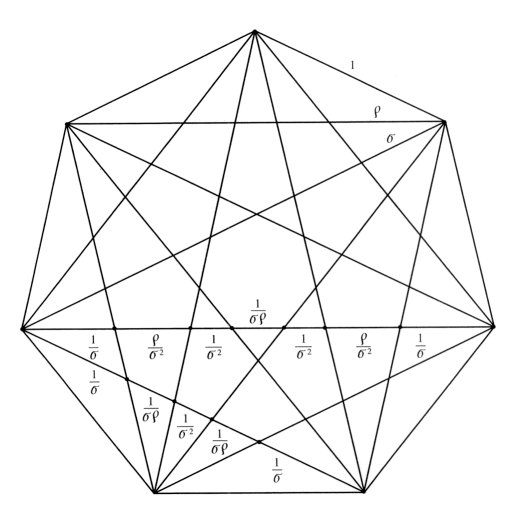
8. The Heptagonal System The heptagonal system is particularly rich in algebraic and geometric relationships. The additive properties of DPF and Table 6 for the heptagon are summarized: r+ s = rs (Compare this with t +t2 = tt2) 1/r + 1/s = 1 (Compare this with 1/t + 1/t2 = 1) r2 = 1 + s s2 = 1 + r + s r /s = r– 1 s /r = s– 1 (7) 1/s = s– r 1/r = 1 + r – s The algebraic properties of each system of proportions are manifested within the segments of the n-pointed star (the n-polygon with all of its diagonals) corresponding to that system. For example, the pentagonal system of proportions is determined by the 5-star while the octagonal system is determined by the 8-star. Figure 7 illustrates the family of star heptagons. Notice that the short diagonal of length r (the edge is 1 unit) and the long diagonal of length s are subdivided into the following segments depending on r and s : r = 1/r + 1/rs + 1/s2 + 1/rs + 1/r and, s = 1/s
+ r /s2
+ 1/s2 + 1/rs
+ 1/s2 + r
/s2 + 1/s
Figure 7
Thus we see at the level of geometry that the graphic designer encounters the same rich set of relationships as does the mathematician at the level of symbols and algebra. The following pair of intertwining geometric s
-sequences and corresponding Fibonacci-like integer series exhibit these
additive properties:
The integer series is generated as follows:
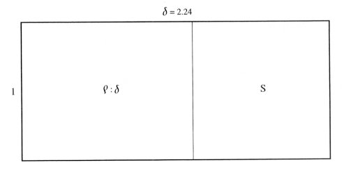
s = 1s + 0r + 0 s2 = 1s + 1r + 1 s3 = 3s + 2r + 1 (9) s4 = 6s + 5r + 3 s5 = 14s + 11r + 6 s6 = 31s + 25r + 14 … Notice that the first coefficient in the equation for sn+1 is the sum of the three coefficients of the equation for sn while the second coefficient is the sum of the first two coefficients and the last coefficient is the same as the first of the previous equation, e.g., in the equation for s 4: 6=3+2+1, 5=3+2, and 3=3. A geometric analogy to the golden mean can be seen by considering the pair of rectangles of proportions r: 1 and s : 1 in Figure 8. By removing a square from each, we are left in both cases with rectangles of proportion r: s although oriented differently. 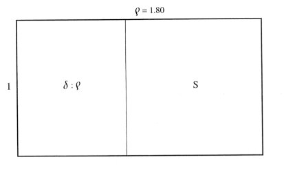
(a)
(b) Figure 8
9. Self-referential Properties of the Silver Mean Constants In general the equation T(x) = x expresses a fixed point or what I refer to as a self-referential relationship. Replacing x by T(x) gives T(T(x)) = x or TTx = x. Continuing this process results in , TTT....Tx = x from which it follows that we can formally set, x = TTT..., an infinite process. For example, if T(x) = –1/x, then setting x = T(x) yields the formal solution, TTT... = –1/–1/–1/–1/... Although this infinite compound fraction has no mathematical meaning, the infinite process can be defined to be the imaginary numbers ±i since these are the solutions to –1/x = x. We now come to a set of self-referential statements related to the SM1 and SM2 constants. These constants are solutions to the self-referential equations T(x) = x where, T(x) = N + 1/x and T(x) = N - 1/x. If N = 0 in the second of these transformations, TTT... is identified with the imaginary number i. So in a sense, the silver means are generalizations of i. The solutions x can be shown to be the two infinite processes, TTT... = N+(1/(1+N/(1+N)))... and TTT... = N-(1/(1-N/(1-N)))... These are continued fraction representations of the silver
mean constants of types 1 and 2. SM1(N) = [N;`N]
in continued fraction notation. SM2(N) = [N;`N]-
are expressed in terms of another form of continued fraction not discussed
in this book.
10. Conclusion With the aid of Pascal’s triangle, the golden mean and
Fibonacci sequences were generalized to a family of silver means. The Lucas
sequence was then generalized with the aid of a close variant of the Pascal’s
triangle. These generalized golden means and generalized F- and
L-sequences
were shown to form a tightly knit family with many properties of number.
Perhaps it is for this reason that they occur in many dynamical systems.
The numerical properties of the silver mean constants are the result of
their self-referential properties which, in turn, derive from their relationship
to the imaginary number i. We have shown that all systems of proportion
are related to a set of polynomials derived from Pascal’s triangle. These
systems are related to both the edges of various species of regular star
polygon and the diagonals of regular n-gons, and they share many
of the additive properties of the golden mean. The heptagon was illustrated
in detail.
Bibliography Kappraff, J., Connections: The Geometric Bridge between Art and Science, 2nd ed., Singapore: World Scientific Publ. (2001). Kappraff, J. , Beyond Measure: A Guided Tour through Nature, Myth, and Number, Singapore: World Scientific Publ. (2002). Ogawa, T., Generalization of the golden ratio: any regular polygon contains self-similarity, in Research of Pattern Formation, ed. R. Takaki, KTK Scientific Publ. (1990). Steinbach, P., Golden fields: A case for the heptagon, Math. Mag. 70(1)(1997). Steinbach, P., Sections Beyond Golden, in Bridges: 2000, ed. R. Sarhangi, Winfield (KS): Central Plains Books (2000). |
 , where h £k.