|
5. Applications Next examples illustrate some applications of Theorems 1 and 4. The first one uses a parameter that allows to change the shape of the attractor continuously. The second example uses affine invariance to gain effects of halftoning prismatic 3D objects. Example 4 (Sierpinski triangle variation). Let Dyz= {(0, 0), (3/4, q/4), (1/4, q/4), (1, 0)} and L ={(0, 0), (3/4, q/4), (1/4, q/4), (1, 0)}, qÎ R. The mappings v1, v2 and v3 are determined by (10)-(11) and by the conditions v1(1/4, q/4) = (1/4, 0), v2(1/4, q/4) = (3/8, 3q/8), v3(1/4, q/4) = (5/8, q/8). Let the IFS s(D) = {R 3; w1, w2, w3}be the lifting of t(Dyz) over the equidistant x-mesh. The yz-projection of its attractor is the Sierpinski triangle. On the other way, preatractors continuously depend on q. The Figure 6 show some preatractors for q = Ö3.
Figure 6. Modified Sierpinski preattractors. Example 5. Here, an application of
the affine invariance property will be given. An example of a space-filling
curve will be modified by the using of Theorem
4. The data set D and the IFS s(D,M)
={R3;
w1,
w2,
w3,
w4} for this example is the same as in Example 2 with this
difference that the line
L is {(0, 0), (1/2,
1), (1, 0)}. The top row of Figure 7 shows preattractors W
1(L),
W
2(L),
W
3(L),
the initial steps in construction of the space filling curve given in Barnsley
[3,
p. 243]. As it is evident from Example
2, is a hyperbolic block diagonal IFS. Let
 (20)
(20)According to Theorem 4, s(D,M) is weakly invariant under the affine mapping w(P) = WP+ v (PÎR3) where v is an arbitrary vector from R3. This means that w(W k(L)) is the same as (W *)k(L*), where W * is the Hutchinson operator associated with the IFS s(w(D),M') and L* = w(L). Here, M'={M1*, M2*, M3*, M4*}, Mi* = NMiN -1, with N = [nij]2x2 being the lower-right diagonal block of W given by (20). The Figure 7 (bottom row) shows preattractors (W *)1(L*), (W*)2(L*) and (W *)3(L*).
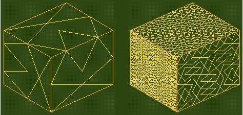
Figure 7. Space filling curve prefractals and their affine images. As we mentioned before, an interesting application of space filling curves in computer graphics is to halftoning and dithering of the images (see [4], [15] ). The next Figure 8 shows how the affine invariance property can be applied in such a case. The same pattern as in Figure 7 is used. The initial data set is affinely transformed to create each face of the "box". The second preattractor from each of the three different Hutchinson orbits is used to draw the cube on the left. This is sufficient for creating the 3D effect. The different shading of the cube faces in the picture on the right is obtained by thicker or lighter filling of the space, corresponding to preattractors at different positions in the Hutchinson orbits corresponding to the single faces.
Figure 8. Space filling combined with affine mappings. |