|
The Golden Section, Fibonacci series and new hyperbolic models of Nature Alexey Stakhov1, Boris Rozin2 The International Club of the Golden Section 6 McCreary Trail, Bolton, ON, L7E 2C8, Canada
Abstract. A survey of new mathematical models of Nature is presented based on the Golden Section and using a class of hyperbolic Fibonacci and Lucas functions, and a surface referred to as the Golden Shofar. Also considered afre generalized Fibonacci numbers, generalized golden proportions, a Generalized Principle of the Golden Section, golden algebraic equations, generalized Binet formulas, generalized Lucas numbers, continuous functions for the generalized Fibonacci and Lucas numbers, Fibonacci matrices, and golden matrices. Key words. The Golden Section, Fibonacci and Lucas numbers, Binet formulas, the Golden Shofar, hyperbolic functions, Dichotomy principle, the Golden Section principle.
1. Introduction One of the major achievements of modern science is an understanding that the world of Nature is hyperbolic. The creator of non-Euclidean geometry was the Russian mathematician Nikolay Lobachevsky who derived a new geometric system based on hyperbolic functions in 1827. The need for new geometrical ideas became apparent in physics at the beginning of the 20th century as the result of Einstein’s Special Theory of Relativity (1905). In 1908, three years after the publication of this great work, the German mathematician Herman Minkovsky gave a geometrical interpretation of the Special Theory of Relativity based on hyperbolic ideas. The theory of hyperbolic functions has developed in ways that, at first sight, does not appear any connection to hyperbolic functions. However, it does not trelate to the theory of Fibonacci numbers, an actively developing branch of modern mathematics [1-3]. In 1993, the Ukrainian mathematicians Alexey Stakhov and Ivan Tkachenko developed a new approach to the theory of hyperbolic functions [4]. Using the so-called Binet formulas, they developed a new class of hyperbolic functions called Hyperbolic Fibonacci and Lucas Functions [4, 5]. This idea was further developed in Stakhov and Rozin’s paper [6], where they defined a class of symmetric Hyperbolic Fibonacci and Lucas functions. The hyperbolic Fibonacci and Lucas functions and the Golden Shofar surface are the most important ingredients of the "golden" mathematical models applicable to the description of the "hyperbolic worlds" of Nature. Also useful for the study of such models are classes of generalized Fibonacci numbers [8], generalized golden proportions [8], golden algebraic equations [9], generalized Binet formulas [10], generalized Lucas numbers [10], continuous functions for the generalized Fibonacci and Lucas functions [11], Fibonacci matrices [12] and golden matrices [13]. These mathematical results were used in algorithmic measurement theory [8, 14, 15], a new theory of real numbers [16], harmony mathematics [17-20], new computer arithmetic [8, 21-23], new coding theory [24-25], and the formulation of the Generalized Principle of the Golden Section [13]. The main purpose of the present article is to give a brief survey of golden mathematical models used for describing the "hyperbolic worlds" of Nature developed by the authors in references [4-25].
2. The Golden Section, Fibonacci & Lucas numbers, and Binet formulas In the "Elements" of Euclid there is a geometric problem to divide a line segment in the extreme and middle ratio. This problem is often called the Golden Section problem [1-3]. the solution of which reduces to the equation:
x2 = x + 1. (1)
Equation (1) has two roots. Its positive root The following expression for the golden ratio follows from Equation (1):
tn = tn-1
+ tn-2 = t´tn-1
(2)
The Fibonacci numbers Fn
= {1, 1, 2, 3, 5, 8, 13, 21, 34, 55, …} (3)
Fn = Fn-1 + Fn-2
(4)
with initial conditions:
F1 = F2
= 1 (5)
The Lucas numbers
Ln
= {1, 3, 4, 7, 11, 18, 29, 47, 76, …} (6)
are another integer sequence given by the recursive
relation:
Ln = Ln-1 + Ln-2
(7)
with initial conditions:
L1 = 1; L2
= 3 (8)
Table 1. The "extended" Fibonacci and Lucas numbers
A number of wonderful mathematical properties of the "extended" series Fn and Ln follow from Table 1. For example, for odd integers n = 2k + 1 the terms of the sequences Fn and F-n coincide, i.e., F2k+1 = F-2k-1, while for even integers n = 2k they have opposite signs, i.e., F2k = -F-2k, whereas the reverse occurs for the Lucas numbers Ln, with L2k = L-2k and L2k+1 = -L-2k-1. There are many fundamental results in
the modern theory of Fibonacci
numbers [1-3]. In the 19th century the famous French mathematician Binet
discovered two remarkable formulas, called the Binet formulas, that
connect Fibonacci (Fn) and Lucas (Ln)
numbers with the golden ratio
Hyperbolic Fibonacci and Lucas functions 3.1. Stakhov and Tkachenko’s approach If we compare Binet formulas (9) and (10) to the classical hyperbolic functions
In [4], the discrete variable k in formulas (9) and (10) was replaced with the continuous variable x that takes its values from the set of real numbers. Consequently, the following continuous functions, which are called the hyperbolic Fibonacci and the Lucas functions, were introduced: The hyperbolic Fibonacci sine
sF(k) = F2k;
cF(k) = F2k+1; sL(k)
= L2k+1;
cL(k) = L2k
, (17)
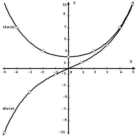
where k is an arbitrary integer.3.2. A symmetrical representation of the hyperbolic Fibonacci and Lucas functions (Stakhov and Rozin’s approach ) Let us compare the hyperbolic Fibonacci and Lucas functions to the classical hyperbolic functions. It is easy to see that, in contrast to the classical hyperbolic functions, the graph of the Fibonacci cosine is asymmetric, while the graph of the Lucas sine is asymmetric relative to the origin of coordinates. This places restrictions on important applications of the new class of hyperbolic functions given by (13)-(16). Based on an analogy between Binet formulas (9) and (10) and the classical hyperbolic functions (11) and (12), the following definitions of the hyperbolic Fibonacci and Lucas functions were given by Stakhov and Rozin’s [6]: Symmetric hyperbolic Fibonacci sine
Symmetric hyperbolic Lucas sine
 ; ;  . (22) . (22)It is easy to construct graphs of the symmetrical Fibonacci and Lucas functions (Fig. 1, 2).
Their graphs have a symmetric form and are similar to
the graphs of the classical hyperbolic functions. However, at the point x=0, the symmetric
Fibonacci cosine cFs(x) takes the value The symmetric hyperbolic Fibonacci and Lucas functions are related to the classical hyperbolic functions and by the identities:
The symmetric hyperbolic Fibonacci and Lucas functions are related among each other by the identities:
3.3. The recursive properties of the symmetric hyperbolic
Fibonacci and Lucas functions
The symmetric hyperbolic Fibonacci and Lucas functions (18)-(21) are generalization of the Fibonacci and Lucas numbers and, therefore, they have recursive properties. On the other hand, they are similar to the classical hyperbolic functions, and therefore they have hyperbolic properties. Table 2 lists the well known identities for Fibonacci and Lucas numbers and the corresponding identities for the symmetric hyperbolic Fibonacci and Lucas functions.
Table 2. The recursive properties of the symmetric
hyperbolic Fibonacci and Lucas functions For example, the famous Cassini formula [26] Fn 2 -
Fn+1 Fn-1
= (-1)n+1, (23)
which is an important identity connecting three adjacent Fibonacci numbers, can be generalized to the symmetric hyperbolic Fibonacci functions as: [sFs(x)]2 - cFs(x+1) ?Fs(x-1) = -1 (24) [cFs(x)]2 - sFs(x+1) sFs(x-1) = 1, (25) It is clear that the identities (24), (25) can be considered
to be generalizations of Cassini formula to continuous functions. 3.4. The hyperbolic properties of the symmetric hyperbolic Fibonacci and Lucas functions Some of the hyperbolic properties of the symmetric hyperbolic Fibonacci and Lucas functions have analogues to the properties of classical hyperbolic functions as shown in Table 3.
Table 3.
The hyperbolic properties of the symmetric
hyperbolic Fibonacci and Lucas functions
For example, the most important identity for the classical hyperbolic functions,
[ch(x)]2 – [sh(x)]2
= 1 (26)
[cFs(x)]2 - [sFs(x)]2
= [cLs(x)]2 - [sLs(x)]2 = 4. (28)
Thus, the above symmetric hyperbolic functions retain all of properties of classical hyperbolic functions (Table 3), while exibiting new new (recursive) properties characteristic of Fibonacci and Lucas numbers (Table 2).Thus, unlike the classical hyperbolic functions, new hyperbolic functions have discrete analogues in the form of Fibonacci and Lucas numbers. According to (22) these functions agree with Fibonacci and Lucas numbers when the continuous variable x takesinteger values. Note that the identities (24) - (28), as well as other identities from Tables 2 and 3, emphasize a fundamental character of the hyperbolic Fibonacci and Lucas functions. We predict that hyperbolic Fibonacci and Lucas functions will have great importance for the future development of Fibonacci and Lucas number theory [1-3]. They generalize Fibonacci and Lucas numbers to the continuous domain since Fibonacci and Lucas numbers are embedded in them. According to Table 2 each discrete identity for Fibonacci and Lucas numbers has its continuous analogue in the form of a corresponding identity for the hyperbolic Fibonacci and Lucas functions, and conversely. Therefore, the theory of the hyperbolic Fibonacci and Lucas functions is more general than traditional Fibonacci and Lucas number theory. This results in the following important consequence: due to the introduction of hyperbolic Fibonacci and Lucas functions, discrete Fibonacci and Lucas number theory [1-3] becomes a part of the continuous theory of hyperbolic Fibonacci and Lucas functions [4-7]! The introduction of hyperbolic Fibonacci and Lucas functions is a new stage in the development of Fibonacci and Lucas number theory.
3.5. Bodnar’s geometry As is well known, Fibonacci and Lucas numbers are the basis of Law of Plant Phyllotaxis " [27]. According to this law, the number of the left and right spirals on the surface of phyllotaxis objects such as the pine cone, pineapple, cactus, head of sunflower, etc. are adjacent Fibonacci numbers, i.e., numbers whose ratios are
These ratios characterize the symmetry of phyllotaxis objects. Thus, for every phyllotaxis pattern is characterized by one of these ratios. This ratio is called the order of symmetry. After observing phyllotaxis patterns
on the surface of a plant, it is natural to wonder how this pattern is
formed during the growth of the plant. This question is at the basis of the
phyllotaxis puzzle which is one of the most intriguing problems of botany.
The key to this puzzle lies in the tendency of bioforms during their growth
to change their symmetry orders according to (29). For example, the florets
of a sunflower at the different levels of the same stalk have different
symmetry orders, that is, the older disks have symmetry orders further out
in the sequence. It means that during growth there is a natural change f the
symmetry order and this change of symmetry is carried out according to the
law:
A change of symmetry orders of phyllotaxis objects according to (30) is called dynamic symmetry [27]. Many scientists feel that the phyllotaxis phenomenon has more general importance. For example, it is Vernadsky ‘s opinion that dynamic symmetry may be applicable to general problems in biology. So, the phenomenon of the dynamic symmetry finds a special role in the geometry of phyllotaxis. We can assume that certain geometrical laws are lurking within the numerical regularity of (30). This phenomenon may be the secret of the phyllotaxis growth mechanism, and its expression could have great importance for the solution of the phyllotaxis problem. The Ukrainian researcher Oleg Bodnar has recently shed light on this problem [27]. Bodnar formulated a geometric theory of phyllotaxis. This theory is based on the hypothesis, that the geometry of phyllotaxis is hyperbolic, and the change of symmetry orders of phyllotaxis objects during their growth is based on the hyperbolic turn, the basic transforming motion of hyperbolic geometry. However, the main feature of Bodnar’s geometry lies in its use of golden hyperbolic functions, which agree with the symmetric hyperbolic Fibonacci and Lucas functions described in this paper up to constant factors. 4. The Golden Shofar 4.1. The quasi-sine Fibonacci function Let us consider the representation of the Binet formula for the Fibonacci numbers in the following form used widely in mathematics [1-3]:
Comparing the Binet formula (31) to the symmetric hyperbolic Fibonacci functions (19) and (20), it follows that the continuous functions txand t-x in the formulas (19) and (20) correspond to the discrete sequences tn and t-nin Equation (31). Consequently it is possible to insert a continuous function into this function that takes the values -1 and 1 at integer values of n analogous to the alternating sequence (-1)n in Binet's formula (31). The trigonometric function cos(px) is the simplest such function. This suggests a new set of continuous functions that are connected to the Fibonacci numbers. Definition 1. The following continuous function is called the quasi-sine Fibonacci function:
TThe graph of the quasi-sine Fibonacci function passes through all points of the coordinate plane corresponding to the Fibonacci numbers (see Fig.3). The symmetric hyperbolic Fibonacci functions (19) and (20) (Fig. 1) are the envelopes of the quasi-sine Fibonacci function . Also the quasi-sine Fibonacci function has recursive properties similar to Fibonacci numbers [7].
Figure 3. The graph of the quasi-sine Fibonacci function
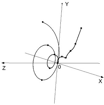
4.2. The three-dimensional Fibonacci spiral
It is well known that the trigonometric sine and cosine
can be defined as projection of the translational movement of a point on
the surface of an infinite rotating cylinder with the radius 1, whose
symmetry center coincides with x-axis.
Such a three-dimensional spiral is projected into the sine function on a
plane and described by the complex function f(x) = cos(x)
+ isin(x), where If we assume that the quasi-sine Fibonacci function (32) is a projection of a three-dimensional spiral on some funnel-shaped surface, then analogous to the trigonometric sine, it is possible to construct a three-dimensional Fibonacci spiral. Definition 2. The following function is a complex representation of the three-dimensional Fibonacci spiral:
CFF(x)
=
4.3 The Golden Shofar Consider real and imaginary parts in the complex Fibonacci spiral: Re[CFF(x)] = Im[CFF(x)] =
y(x) - z(x) = Square both expressions of system (37) and add them, taking y and z as independent variables, to get the following curvilinear surface. Definition 3. The three-dimensional curved surface given by,
 + z2
= + z2
=  . (38) . (38) is called the Golden Shofar and
shown in Fig. 5.
Figure 5. The Golden Shofar
Formula (38) for the Golden Shofar can also be represented in the form:
z2 = [cFs(x) –
y][sFs(x) + y], (39)
4. A general model of the hyperbolic space with a "shofarable" topology Based on experimental data obtained in 2003 by the NASA's Wilkinson Microwave Anisotropy Probe (WMAP), a new hypothesis about the structure of the Universe was developed. According to [28], the geometry of the Universe is similar in shape to a horn or a pipe with an extended bell [27]. As a result of this disclosure we make the following claim: The Universe has a "shofarable" topology as shown in Fig.6.
Figure 6. The "shofarable" topology 6. A further development of the "golden" mathematical models 6.1. Fibonacci p-numbers Reference [8] introduces generalized Fibonacci numbers related to Pascal's triangle. For a given p=0, 1, 2, 3, ... generalized Fibonacci numbers are given by following recursive relation:
Integer sequences corresponding to the formulas (40), (41) are called Fibonacci p-numbers [8]. We have proved that Fibonacci p-numbers can be expressed in terms of the binomial coefficients as follows [8]:
Note that expressions (40) and (41) create an infinite number of new recursive numerical sequences since every р generates its own numerical sequence. In particular, р=0 generates the binary sequence: 1, 2, 4, 8, 16, 32, ... , while for р=1 the classical Fibonacci sequence (3) results. For the case р=0 Equation (42) takes the form
6.2.The golden p-proportions and the "golden" algebraic equations It is well known that the ratios of adjacent Fibonacci numbers Fn/Fn-1 approach the golden mean in a limiting sense. We have also shown that the ratio of adjacent Fibonacci р-numbers Fp(n)/Fp(n-1) approaches in the limit some positive number tp that is a positive root of the polynomial equation [8] xp+1
= xp + 1,
(45)
where p=0, 1, 2, 3, … .
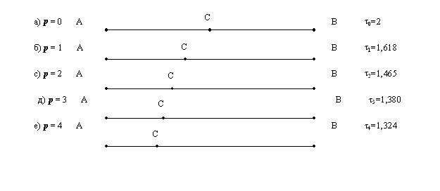
The numbers tp are referred to as golden р-proportions since for the case р=1 the number tp coincides with the classical Golden Proportion. We call Equation (45) the golden algebraic equation because for the case р=1 Equation (45) reduces to Equation (1) [9] Note that for the case p=0, tp=t0 =2 and for the case p=¥, tp= t¥ =1. This means that on the number line between the numerical constants 1 and 2 there are an infinite number of numerical constants tp, which expresses some deep mathematical properties of Pascal triangle. We have formulated the following geometric problem called a problem of the golden p-section. Consider a given integer р=0, 1, 2, 3, ..., and divide a line segment AВ by a point C according to the following relation also shown in Fig. 7:
Figure 7. The Golden p-sections (p = 0, 1, 2, 3, ...) A solution to problem (46) to find a section point C of line segment AB reduces to a search for a positive root of the Equation (45), i.e., the division of a line segment according to Equation (46) is equal to the golden р-proportion [8]. Consider two cases of the golden р-section: for the case р=0 the golden р-section reduces to a bisection (Fig. 7а), while for the case p = 1 it reduces to the classical golden section (Fig. 7b). For the remaining values of р we get an infinite number of proportional divisions of the line segment according to Relation (46). In particular, it is easy to show that for the case p®¥, tp® 1. The following identity relating powers of the golden р-proportion degrees follows directly from (45):
Equation (45), being the equation for the roots of a (p+1)-th degree polynomial, has p+1 roots x1, x2, x3, …, xp, xp+1. Later we show that the root x1 always coincides with the golden p-proportion tp, i.e., x1 = tp. Also each of the roots x1, x2, x3, …, xp, xp+1 satisfies Equation 47,
The roots of Equation (45) satisfy the following identities [9]: x1+x2+x3+x4+... +xp+xp+1 =1 (49) x1x2x3x4...xp-1xpxp+1 = (-1) p (50)
x1k
+
x2k
+
x3k
+
x4k+...
+xpk
+ xp+1k = 1. (51)
We have proved that there are an infinite number of the golden algebraic equations that are derived from equation (45):
Note that Equations (52) have a common root tp. In particular, for the case p=1 a general equation (52) takes the form: xn = Fnx + Fn-1, (53)
where Fn, Fn-1 are Fibonacci numbers.
For the case n=4 Equation (53) takes the form: x4 = 3x +
2. (54)
Equation (54) leads to the unexpected result that it describes the energy levels of the molecule butadiene, a chemical used for rubber production. The famous American physicist, Richard Feynman, expressed his admiration for Equation (54) with the following remark: "What miracles exist in mathematics! According to my theory, the Golden Proportion of the ancient Greeks gives the condition for the minimal energy of the butadiene molecule.” This connection to chemistry raises our level of interest in the golden algebraic equations. Perhaps these equations could be used to model the energy conditions of other molecules. 6.3. The Generalized Principle of the Golden Section Consider the main identity for the golden p-proportion given by (47), and divide all terms by to get the following identity for a “unit”:
 (56) (56)
Note that for р=0 Equation (57) takes the following form: Finally, for p=1 identity (57) takes the following form: Thus, identity (57) defines a more general principle for dividing a line segment into two parts, referred to in [13] as the “Generalized Principle of the Golden Section” for which the “Dichotomy Principle” and the “Golden Section Principle” are sub-cases.
6.4. The generalized Binet formulas and the continuous functions for the Fibonacci and Lucas p-numbers Generalized Binet formulas enable Fibonacci p-numbers to be expressed in analytic form [10]. For a given integer p>0 any Fibonacci p-number Fp(n) (n=0, ±1, ±2, ±3, …) can be be represented in terms of the roots of the golden algebraic Equation (46) in the following form:
Fp (n) =
k1(x1)n
+ k2(x2)n + … + kp+1(xp+1)n
(60)
where k1, k2,
… , kp+1 are constant coefficients that are solutions of
the following system of algebraic equations:
In particular, for р=1 the Fibonacci р-numbers reduce to the classical Fibonacci numbers Fn . For this special case expression (60) reduces to the well-known expression [2, 3]:
Fn =
k1(x1)n + k2(x2)n,
(62)
x1 =
where,
k1 =
 .
(66) .
(66)It has been shown that Lucas numbers Ln can be expressed in terms of the roots x1, x2 in the following form: [2, 3] We have shown [10] that the sum of the n-th powers of the roots x1, x2, …, xp+1 of the Equation (45) establishes a new class of recursive sequences referred as Lucas р-numbers Lp(n), where p=0, 1, 2, 3, ..., i.e., Lp (n) = (x1)n + (x2)n
+ … + (xp+1)n
(68)
Using properties (48)-(51) of
Equation (46) series (68) follows from the recursive relation:
Lp (n) = Lp (n-1) + Lp
(n-p-1) (69)
with the following initial terms: Lp (0) = p+1 (70) Lp (1) = Lp(2) = ... = Lp (p) = 1. (71)
Table 4. Lucas p-numbers
Thus, the main result of reference [10] ] is a generalization of the Binet formulas and the development of a new class of recursive numerical sequences, the generalized Lucas numbers or Lucas p-numbers, given either in analytical form (68) or in recursive form (69)-(71). These new recursive numerical sequences are of great theoretical interest, and they may prove useful for the characterization of certain natural processes. As shown above, hyperbolic Fibonacci
and Lucas functions (13)-(16) and (18)-(21) are generalizations of the Binet
formulas (9)-(10) to the continuous domain [11]. The
generalized Binet formulas (60), (68), which allow us to express the Fibonacci
and Lucas р-numbers in terms of the roots of Equation (45), can be used to
define continuous functions for the Fibonacci and Lucas р-numbers as was done
for hyperbolic Fibonacci and Lucas functions. The equations for the continuous
functions of the Fibonacci and Lucas p-numbers are more complex than Equations
(13)-(16) and (18)-(21). Nevertheless, the results of article [11]
can be considered to be a variant of the golden hyperbolic models of Nature with
the potential to be useful in the natural sciences.
6.5. Fibonacci matrices Over past few decades, the theory of Fibonacci numbers has been complemented by the theory of the Fibonacci Q-matrix [7]. The latter is a square 2´2 matrix of the following form: Det Q = -1. (73)
 , (74) , (74)Using (73), it is easy to get the following expression for the determinant of matrix (74):
where n is an integer. On the other hand, the determinant of matrix (74) is given by
The idea of the Q-matrix was developed in [12], where the following square (p+1)´(p+1) Qp-matrix was introduced:
for p = 0, 1, 2, 3, … It contains a p´ p-identity matrix identity matrix bordered by the last row, which consists of 0’s and a leading 1, and the first column, which consists of 0’s embraced by a pair of 1’s. We list the Qp-matrices for p = 0, 1, 2, 3, 4: Q0 = (1) ;
The main result of reference [12] is a proof of the following expression for the n-th power of the Qp-matrix:
where p =0, 1, 2, 3, …, n = 0, ± 1, ± 2, ± 3, …, and elements of the matrix are the Fibonacci p-numbers. Note that the class of matrices (77) has an interesting recursive property. If we cross out the last, that is, (p+1)-th column and the next to the last, that is, p-th row in the Qp-matrix, then the matrix reduces to matrix Qp-1. This means that the determinant of the Qp-matrix differs from the determinant of the Qp-1-matrix only by its sign, i.e., Det Qp-1
= - Det Qp . (79)
Det Qp = (-1)p.
(80)
Det
where p = 0, 1, 2, 3, … ; n = 0, ±
1, ± 2, ±
3, … .
The main result of reference [12] is the development of a new class of square matrices satisfying Equation (81). It is clear that matrices (77) and (78) can be used for the future progress of Fibonacci research. Here expression (81) can be considered to be a generalization of the “Cassini formula” . For example, for the case р=2 the generalized “Cassini formula” takes the form: Det + F2(n-1)[F2(n-1)F2(n-1)
- F2(n)F2(n-2)] = 1. (82)
There are an infinite number of generalized Cassini formulas similar to (82) for р=1, 2, 3, ...
6.6. The "golden" matrices Stakhov has introduced a class of golden matrices [13]. Let us represent matrix (74) in the form of two matrices, one for even (n=2k) and the other for odd (n=2k+1) values of n:
Substituting discrete variable k in the matrices (85), (86) with continuous variable x, results in two unusual matrices that are functions of x:
It is clear that the matrices (87), (88) are generalizations
of the Q-matrix (74) for the continuous domain. These matrices have a
number of unusual mathematical properties. For example, for  (89)
(89)Using properties (24) and (25) of the symmetric hyperbolic functions to compute the determinants of matrices (87) and (88) leads to the result, Det Q2x = 1 (90) Det Q2x+1 = - 1 (91) Therefore these determinants are independent of x and equal identically to 1 in absolute value. In fact identities (90) and (91) are generalizations of the Cassini formula to the continuous domain! At present it is difficult to predict where matrices (78), (87), (88), having unusual mathematical properties (79), (81),(90), (91), might be used. However, they were recently applied to coding theory and cryptography [13, 24, 25].
4. Conclusion References [4-25] have been successful in developing new mathematical equipment, based on both the classical golden section and the golden p-sections, useful for describing the “hyperbolic worlds” of Nature. The most important of these golden mathematical models are the following: 1. Hyperbolic Fibonacci and Lucas functions. A consequence of their introduction has been the realization that the classical hyperbolic functions (12), (13), which are useful in mathematics and theoretical physics, are not the only tools for creating mathematical models of the “hyperbolic world". In addition to models based on classical hyperbolic functions (Lobachevsky's hyperbolic geometry, Minkowsky’s geometry, etc.), there is a golden hyperbolic world based on hyperbolic Fibonacci and Lucas functions[4-7]. The golden hyperbolic world exists objectively and independently of our awareness. This “hyperbolic world” is ubiquitous to Living Nature. In particular, it appears in pinecones, sunflower heads, pineapples, cacti, and in florescence’s of various flowers in the form of the Fibonacci and Lucas spirals on the surfaces of these biological objects (the phyllotaxis law). Note that the hyperbolic Fibonacci and Lucas functions [4-7], which underlie phyllotaxis phenomena are not mere inventions of Fibonacci-mathematicians, but rather they objectively reflect the mathematical laws underlying the geometry of Living Nature. 2. The Golden Shofar. The Golden Shofar is another new model of the golden hyperbolic world. The article «Hyperbolic Universes with a Horned Topology and the CMB Anisotropy» [28] proved a great surprise to the authors because it showed that the geometry of the Universe is quite possibly is “shofarable” by its structure. 3. The Generalized Principle of the Golden Section, which is based on the golden р-proportions, is of general scientific interest and could influence the development of all natural sciences wherever the “Dichotomy Principle” and the classical Golden Section Principle are used [29]. In summary, the authors would like to express their surprise that it has taken so long for mathematicians and physicists to give proper attention to the development of the mathematical needed to model the golden hyperbolic world. However, toward the end of the 20th century, due to the efforts of several theoretical physicists, the situation began to change. References [30-39] demonstrate a substantial interest on the part of modern theoretical physicists in the golden section and the golden hyperbolic world. The works of Shechtman, Butusov, Mauldin and William, El Naschie, Vladimirov, Petoukhov and other scientists show that it is impossible to imagine future progress in physical and cosmological research without a consideration of the golden section. In this connection, the golden genomatrices of the Russian scientist Sergey Petoukhov [39] are of great importance for the future development of science. Petoukhov’s discovery shows that the golden section underlies the genetic code! It seems that the dramatic history of the golden section, which has continued over several millennia, may conclude with a great triumph for the golden section in the beginning of the 21st century, the “Century of Harmony.” Penrose tiles, a resonance theory of the Solar system (Molchanov and Butusov ), quasi-crystals (Shechtaman), fullerenes (Kroto, Curl and Smalley, 1996 Nobel Prize in chemistry) were only precursors of this triumph. “Harmony Mathematics” (Stakhov), hyperbolic Fibonacci and Lucas functions (Stakhov, Tkachenko, Rozin), Bodnar’s geometry, the “Law of structural harmony of systems” (Soroko), El Nashie’s theory of E-infinity, Fibonacci matrices and a new coding theory (Stakhov), the golden matrices and a new cryptography (Stakhov), and finally the golden genomatrices (Petoukhov) are only a partial list of recent scientific discoveries based on the golden section. These discoveries give reason to suppose that the golden section may be a kind of “metaphysical knowledge”, “pre-number”, or “universal code of Nature”, which could become the foundation for the future development of science, in particular, mathematics, theoretical physics, genetics, and computer science. In 1996, The Fibonacci Quarterly, published the paper “On Fibonacci hyperbolic trigonometry and modified numerical triangles” written by the well-known Fibonacci-mathematician Zdzislaw W. Trzaska [40]. On the one hand, interest of Fibonacci-mathematicians in hyperbolic Fibonacci functions should be encouraged, on the other hand a comparison of Trzaska’s paper [40] and Stakhov and Tkachenko’s paper [4] showed that, in the part concerning hyperbolic Fibonacci functions, Trzaska used all of the material of Stakhov and Tkachenko’s paper [4] without attribution thus creating the perception that he was the original discoverer of the hyperbolic Fibonacci functions. However, since reference [4] was published in 1993, three years before the publication of Trzaska’s paper, this establishes Stakhov and Tkachenko’s priority in the discovery of hyperbolic Fibonacci and Lucas functions.
References [1] Vorobyov N.N. Fibonacci Numbers. Moscow: Nauka, 1978 [in Russian] [2] Hoggat V.E. Fibonacci and Lucas Numbers. - Palo Alto, CA: Houghton-Mifflin; 1969. [3] Vajda S. Fibonacci & Lucas Numbers, and the Golden Section. Theory and Applications. - Ellis Horwood limited; 1989. [4] Stakhov A.P, Tkachenko I.S. Hyperbolic Fibonacci trigonometry. – J Rep Ukrainian Acad Sci, 1993; 208 (7); 9-14 [in Russian] [5] Stakhov A.P. Hyperbolic Fibonacci and Lucas Functions: a new mathematics for the living nature. Vinnitsa: ITI; 2003. ISBN 966-8432-07-X. [6] Stakhov A, Rozin B. On a new class of hyperbolic function. Chaos, Solitons & Fractals 2004, 23(2): 379-389. [7] Stakhov A., Rozin B. The Golden Shofar . Chaos, Solitons & Fractals 2005, 26(3); 677-684. [8] Stakhov A.P. Introduction into algorithmic measurement theory. Moscow: Soviet Radio, 1977.[9] Stakhov A., Rozin B. The "golden" algebraic equations. Chaos, Solitons & Fractals 2005, 27 (5): 1415-1421. [10]. Stakhov A., Rozin B. Theory of Binet formulas for Fibonacci and Lucas p-numbers. Chaos, Solitons & Fractals 2005, 27 (5): 1162-1177. [11] Stakhov A., Rozin B. The continuous functions for the Fibonacci and Lucas p-numbers. Chaos, Solitons & Fractals 2006, 28 (4): 1014-1025. [12] Stakhov A.P. A generalization of the Fibonacci Q-matrix . J Rep Ukrainian Acad Sci 1999, No 9: 46-49. [13] Stakhov A. The Generalized Principle of the Golden Section and its applications in mathematics, science, and engineering. Chaos, Solitons & Fractals 2005, 26 (2): 263-289. [14] Stakhov A.P. Algorithmic measurement theory. ?oscow: Znanie 1979. [15] Stakhov A.P. The Golden Section in the measurement theory. An International Journal "Computers & Mathematics with Applications" 1989, Vol.17, No 4-6: 613-638. [16]. Stakhov A.P. Generalized Golden Sections and a new approach to geometric definition of a number. Ukrainian Mathematical Journal 2004, 56 (8): 1143-1150. [17] Stakhov A.P. The Golden Section and Modern Harmony Mathematics. Applications of Fibonacci Numbers 1998, Vol. 7: 393-399. [18] Stakhov A.P. Sacral Geometry and Harmony Mathematics. Moscow: Academy of Trinitarism, Electronic publication, ? 77-6567, published 11176, 26.04.2004. [19] Stakhov A.P. Harmony Mathematics as a new interdisciplinary direction of modern science. Moscow: Academy of Trinitarism, ? 77-6567, publication 12371, 19.08.2005 [20] Stakhov A. Fundamentals of a new kind of Mathematics based on the Golden Section. Chaos, Solitons & Fractals 2005, 27 (5): 1124-1146. [21] Stakhov A.P. Codes of the Golden Proportion. Moscow: Radio and Communications 1984. [22] Stakhov A.P. Brousentsov’s ternary principle, Bergman’s number system and ternary mirror-symmetrical arithmetic. The Computer Journal 2002, Vol. 45, No. 2: 222-236. [23] Stakhov A.P. Brousentsov’s ternary principle, Bergman’s number system and the :golden" ternary mirror-symmetrical arithmetic. Moscow: Academy of Trinitarism, ? 77-6567, publication 12355, 15.08.2005 [in Russian] [24] Stakhov A., Massingue V., Sluchenkova A. Introduction into Fibonacci coding and cryptography. Kharkov: Publisher "Osnova" 1999. ISBN 5-7768-0638-0. [25] Stakhov A.P. Data coding based on the Fibonacci matrices. Proceedings of the International conference "Problems of Harmony, Symmetry and the Golden Section in Nature, Science, and Art" Vinnitsa: Vinnitsa State Agricultural University 2003: 311-325. [26] Stakhov A.P. Cassini formula. Moscow: Academy of Trinitarism, ? 77-6567, publication 12542, 01.11.2005. [27] Bodnar O.Y. The Golden Section and non-Euclidean geometry in Nature and Art. Lvov: Svit 1994 [in Russian]. [28] Aurich R., Lusting S., Steiner F., Then H. Hyperbolic Universes with a Horned Topology and the CMB Anisotropy. Classical Quantum Gravity 2004, No. 21: 4901-4926. [29] Shevelev I.S. Meta-language of the Living Nature. Kostroma: Voskresenie 2000 [in Russian].[30] Gratia D. Quasi-crystals. Uspechi physicheskich nauk 1988, Vol. 156: 347-363 [in Russian] [31] Butusov K.P. The Golden Section in the Solar System. Problemy issledovania vselennoi 1978, ?7: 475-500. [32] Mauldin R.D and Willams SC. Random recursive construction . Trans. Am. Math. Soc., 1986, 295: 325-346. [33] El Naschie M.S On dimensions of Cantor set related systems. Chaos, Solitons & Fractals 1993, 3: 675-685 [34] El Nashie M.S. Quantum mechanics and the possibility of a Cantorian space-time. Chaos, Solitons & Fractals 1992, 1: 485-487 [35] El Nashie M.S. Is Quantum Space a Random Cantor Set with a Golden Mean Dimension at the Core? Chaos, Solitons & Fractals 1994, 4(2): 177-179 [36] El Naschie M.S. Elementary number theory in superstrings, loop quantum mechanics, twistors and E-infinity high energy physics. Chaos, Solitons & Fractals 2006, 27(2): 297-330. [37] Vladimirov Y.S. Quark icosahedron, charges and Vainberg’s angle. Proceedings of the International conference "Problems of Harmony, Symmetry and the Golden Section in Nature, Science, and Art" Vinnitsa: Vinnitsa State Agricultural University 2003: 69-79.[38] Vladimirov Y.S. Metaphysics. Moscow: Binom
2002. [40] Trzaska Z.W. On
Fibonacci hyperbolic trigonometry and modified numerical triangles. Fib. Quart.
1996, 34, 129-138. |
||||||||||||||||||||||||||||||||||||||||||||||||||||||||||||||||||||||||||||||||||||||||||||||||||||||||||||||||||||||||||||||||||||||||||||||||||||||||||||||||||||||||||||||||||||||||||||||||
 ,
(9)
,
(9)
 . (10)
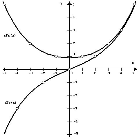
 ;
;
 ;
;  .
.
 (83)
(83)
 (84)
(84)