Three “key” problems of mathematics on
the stage of its origin,
the “Harmony Mathematics” and its
applications in contemporary mathematics, theoretical physics and computer
science
Аlexey Stakhov
The International Club of the Golden Section
6 McCreary Trail,
goldenmuseum@rogers.com · www.goldenmuseum.com
Abstract
We
develop a new approach to the history of mathematics based on the three “key”
ideas of mathematics on the stage of its origin: a count, a measurement
and a harmony. Two
first ideas resulted in the substantiation of two
fundamental mathematical concepts, natural numbers and irrational
numbers, and to the creation of number theory and measurement
theory that underlie “classical mathematics”. The “harmony idea”
connected with the “golden mean” underlies the Harmony Mathematics,
the alternative direction of the mathematics development. We claim that the
Harmony Mathematics will
become a fruitful source for the development of many fundamental theories of
contemporary mathematics, theoretical physics and computer science.
Algebra
and Geometry have one and the same fate. The very slow successes did follow after the fast ones at the
beginning. They left science in the state very far from perfect. It happened,
probably, because mathematicians paid the main attention to the higher parts of the
Analysis. They neglected the beginnings and did not wish to develop
those fields, which they finished once and left them from behind.
Nikolay
Lobachevsky
1. Introduction.
On the
stage of the mathematics origin its development was stimulated by three “key”
problems: a count, a measurement, and a harmony. The two
first problems resulted in the substantiation of the fundamental mathematical
concepts, natural numbers and irrational numbers, and to the
creation of two fundamental mathematical
theories, number theory and measurement theory. These fundamental
concepts and theories underlie “classical mathematics”, “classical theoretical
physics”, and “classical computer science”.
The “Harmony problem” connected with
the “golden mean” was
ignored in every possible way by the “materialistic” science and “classical
mathematics” and this scientific area was developing in the isolation from the
“classical science”. And only on the boundary of the 20th and 21st
centuries the “Harmony Mathematics”, which takes its origin in “The Elements”
of
The main purpose of the present article is to consider a history of mathematics from the point of view of its “key” problems on the stage of its origin and to substitute the “Harmony Mathematics” as a new interdisciplinary direction, which has a direct relation to contemporary mathematics, theoretical physics and computer science.
Part 1. A new approach to the history of
mathematics from the point of view
of
its “key” problems
2. The basic stages in mathematics progress
What is
mathematics? To answer this question we will address to the book “Mathematics
in its historical development” [90], written by the outstanding Russian
mathematician, academician Andrew Kolmogorov. According
to Kolmogorov's definition, mathematics is "a science about
quantitative relations and spatial forms of
real world".
Kolmogorov writes that "the
clear understanding of mathematics as a special science, which have the own subject and method, did arise
for the first time in the Ancient
Kolmogorov points out the following
stages in mathematics development:
(1) Period
of the “mathematics origin”,
which preceded the Greek mathematics.
(2) The
“Elementary mathematics” period.
This period started to develop at 6-5 centuries BC and was ended in 17th
century. The volume of mathematical knowledge obtained before the beginning of
17th century is until now the base of the "Elementary
mathematics", which is taught in secondary and high school.
(3) The “Higher
mathematics” period,
which began with the use of variables in Descartes’ analytical geometry and the
creation of differential and integral calculus.
(4) The
“Modern mathematics” period. Lobachevski’s
“imaginary geometry” is considered as the beginning of this period.
Lobachevski’s geometry gave the beginning of the expansion of the circle of the
quantitative relations and spatial forms, which start to be investigated by mathematics. The development of
similar kind of mathematical researches gave mathematics many new important
3. The “count” problem is the first "key" problem of the ancient
mathematics
In the period of the mathematics
origin Kolmogorov points out some "key" problems, which did stimulate
the development of mathematics and occurrence of its fundamental concepts. The “count” problem is the first of them.
It is emphasized in [90] that "on
the earliest steps of the culture development a count of things resulted in the
creation of the elementary concepts of natural numbers arithmetic. Only on the
base of the developed system of the oral notation, the written notations arose
and different methods of the fulfillment of four arithmetical operations for
natural numbers were gradually developed”.
In
the period of the mathematics origin one of the "key" mathematical
discoveries was made. We are talking about the positional principle of
numbers representation. It is emphasized in [91] that "the
Babylonian sexagecimal numeral system, which arose approximately at 2000 BC,
was the first numeral system based on the positional principle". This
discovery underlies all early numeral systems created during the period of the "mathematics origin" and the "Elementary mathematics" period (including decimal system
and binary system).
Everybody
can agree with the statement that all people after graduating from secondary
school should know at least two useful things: how to read and write and how to
use decimal arithmetic to perform elementary arithmetic operations. The decimal
system, or numeral system for any other base, is one of the milestones of human
intellect. All these
numeral systems are based on the "positional principle” suggested by the
Babylonians. While the decimal system seems to us to be so simple and
elementary, it could be difficult for some people to agree with the statement
that the decimal system and “positional principle” are the greatest mathematical
discoveries. To prove the validity of this statement we can address to the
opinion of the authoritative mathematicians.
Pierre-Simon Laplace (1749-1827), the great French mathematician,
member of the Parisian academy of sciences, an honorable foreign member of the
"The idea to express all numbers
by 9 numerals, betraying to them, apart from the significance by their form,
another significance by their position too, is so simple, that because of this
simplicity it is difficult to understand how this idea is surprising. How not easy to find
this method, we can see on the example of the greatest geniuses of Greek
science Archimedes and Apollonius, from whom this idea remained latent."
M.V. Ostrogradsky (1801-1862), the Great Russian
mathematician, a member of the
“It seems to us that after the
invention of the written language the use by humanity of the so-called decimal notation
is the greatest discovery. We want to say that the agreement, with the aid of
which we can express all the useful numbers by twelve words and their endings
is one of the most remarkable creations of human genius…”.
Jules Tannery
(1848-1910), the French mathematician, a member of the Parisian academy of
sciences:
“The present system of the written notation,
which uses 9 significant numerals and a zero digit and relative significance of
digits, defined by a special rule, had
been introduced in
It is necessary to note that the positional principle of number representation and positional numeral systems (in particular, binary system created at the period of the mathematics origin), became one of the "key" ideas of modern computer science. In this connection it is necessary to remind also, that algorithms of multiplication and the divisions of numbers, used in modern computers, were created by the ancient Egyptians (the method of doubling) [91]. However, the main result of arithmetic's development in the period of the mathematics origin is the formation of natural number's concept, which is one of the major and fundamental mathematical concepts, without which the existence of mathematics is impossible. For studying the properties of natural numbers during the ancient period the number theory, one of the fundamental mathematical theories, did arise.
3. The “measurement” problem is the second
“key” problem of the ancient mathematics
The
“measurement” problem is the second “key” problem, which stimulated the
mathematics development at the period of its origin. Kolmogorov emphasizes in [90],
that "the needs of
measurement (of quantity of grain, length of road, etc.) resulted in the
occurrence of the names and designations of the elementary fractions and to the
development of the methods of the fulfillment of arithmetic operations for
fractions ... The measurement of areas and volumes, the needs of the building
engineering, and a little bit later the needs of astronomy caused the
development of geometry".
A discovery of the “incommensurable line segments” is
a “key” discovery in this area. This discovery was made at 5th century BC in Pythagoras’
scientific school at the investigation of the ratio of the diagonal to the side
of a square. Pythagoreans proved that this ratio cannot be represented in the
form of the ratio of two natural numbers. Such line segments were named
incommensurable, and the numbers representing similar ratios were named
“irrational”. A discovery of the "incommensurable line segments"
became a turning point in the development of mathematics. Owing to this
discovery a concept of irrational number, the second (after natural
numbers) fundamental concept of mathematics, came into mathematics. .
For
overcoming the first crisis in the bases of mathematics, caused by the discovery
of "incommensurable line segments", the Great mathematician Eudoxus
developed a theory of
magnitudes, which was transformed later into mathematical measurement
theory [92, 93]. The measurement theory became one more fundamental theory
of mathematics. This theory underlies all “continuous mathematics” including
differential and integral calculus.
The
influence of the "measurement” problem on the development of mathematics was
so great, that the famous Bulgarian mathematician, academician L. Iliev proclaimed that "during the first epoch of the
mathematics development, from antiquity to the discovery of differential and
integral calculus, mathematics, by investigating first of all the measurement problems, had
created Euclidean geometry and number theory" [94].
Thus,
two "key" problems of the ancient mathematics, the “count” problem
and the “measurement” problem, resulted in the formation of two fundamental
concepts of mathematics, natural numbers
and irrational numbers, which
together with number theory, positional numeral systems, and measurement theory became the base of
“classical mathematics”, “classical theoretical physics” and “classical
computer science”.
4. The “Harmony problem” in its historical
development
4.1. A
division in the extreme and mean ratio
However,
there was one more "key" problem in the ancient science. This problem
played a fundamental role in the development of science, including,
mathematics. We are talking about the "Harmony” problem, which, since the
Greek period, was in the focus of research thought. The first mathematical
methods of the proportion expression in the natural systems appeared in this
period. The formulation of the problem of the division in the extreme and
mean ratio is the “key” discovery in this area. Later this division was
named the golden section. The Great Russian philosopher
Alexey Losev wrote in [95]: "From Plato’s point of view and generally
from the point of view of all antique cosmology,
the Universe is the certain proportional whole that is subordinated
to the law of harmonic division, the Golden Section".
In this
connection it is pertinently to consider "The Elements” of
During its historical development the “classical
mathematics" did lose Pythagoras and Plato’s "harmonic idea" embodied
by
4.2.
Fibonacci numbers
Nevertheless,
despite of negative attitude of "materialistic" mathematics to the
"golden mean", its theory continued to develop. The famous Fibonacci
numbers 1, 1, 2, 3, 5, 8, 13, 21, 34, …can be considered as very
important step in the development of the Harmony Mathematics. They were introduced into mathematics at
13th century by the Italian mathematician Leonardo from
4.3. The first book on the Golden
Mean in the history of science
During
the Italian Renaissance the interest in the “golden mean" arises with new force.
Of course, the universal genius of the Italian Renaissance Leonardo da Vinci
could not pass past the "division in the extreme and mean ratio” (the
"golden section"). There is an opinion [18] that Leonardo had
introduced into the Renaissance culture the name of the "golden
section". Leonardo da Vinci’s did
influence on the book "Divina Proportione" [1], which was published
by the outstanding Italian mathematician Luca Paccioli in 1509. This unique
book was the first book on the golden mean in world history. The book was
illustrated by the 60 brilliant figures drawn by Leonardo da Vinci and influenced on the Renaissance culture
4.4. Johannes Кеплер and the golden section
At 17th
century the Great astronomer and mathematician Johannes Kepler created an
original geometrical model of Solar system based on the Platonic Solids. He did
express the admiration by the golden section in following words: “Geometry has two great treasures: the first
one is Pythagoras’ Theorem; the other, the division of a line into extreme and
mean ratio. We may compare the first one to a measure of gold; we may name the
second one a precious stone”.
4.5. The researches by Lucas, Binet and Felix Klein
After
Kepler's death the interest in the golden section, one of two "treasures
of geometry", decreases for some reasons. And such strange oblivion
continued during two centuries. An active interest in the golden section again
revives in the mathematics only at 19th century. During this period
the mathematical works, devoted to Fibonacci numbers and the golden section,
according to the witty saying of one mathematician, "start to reproduce
as Fibonacci’s rabbits". The French mathematicians Lucas and Binet
become the leaders of these researches in 19th century. Lucas
introduced into mathematics the name of the "Fibonacci numbers",
and also a concept of the "generalized Fibonacci sequences". The
Lucas numers
1, 3, 4, 7, 11, 18.... were
one of them. Binet derived the well-known Binet formulas, which united
the golden mean with the Fibonacci
and Lucas numbers.
In 19th century the outstanding German mathematician Felix Klein tried to unite all branches of mathematics on the basis of the icosahedron, the Platonic Solid, dual to the dodecahedron [96]. Klein treats the icosahedron, based on the golden section, as the geometrical object, from which the branches of five mathematical theories follow: geometry, Galois theory, group theory, invariants theory, and differential equations. Klein's main idea is extremely simple: "Each unique geometrical object is connected with the icosahedron properties". Unfortunately, this unique idea did not be developed in mathematics until now.
4.6. The golden section and Fibonacci
numbers in mathematics of 20th century
In the second half of 20th century the interest in Fibonacci numbers and the golden mean in mathematics was reviving with new force. The prominent mathematicians Gardner [5], Vorobyov [6] Coxeter [7], Hoggatt [9] were the first researchers who felt new tendencies in mathematics. In 1963 the group of the American mathematicians organized the Fibonacci Association and started to issue "The Fibonacci Quarterly". Owing to the activity of the Fibonacci Association and the publications of the special books by Vorobyov [6], Hoggatt [9], Vaida [21], Dunlap [31] and other mathematicians, a new mathematical theory, the “Fibonacci numbers theory”, appeared in contemporary mathematics. This theory has own interesting mathematical history what is shown in the book “A Mathematical History of the Golden Number” written by the prominent Canadian mathematician Roger Herz-Fishler [33].
In
1992 the group of of the Slavic scientists from
4.7. The modern scientific discoveries based on
the Golden Mean and Platonic Solids
The golden mean, pentagram and Platonic Solids were widely used by astrology and other esoteric sciences, what became one of the reasons of the negative attitude of the "materialistic" science to the golden mean and Platonic Solids. However, all attempts of the "materialistic" science and mathematics to forget the "golden mean" and Platonic Solids and to throw out them together with astrology and esoteric sciences on the "dump of the doubtful scientific concepts", had failed. Mathematical models based on the golden mean, Fibonacci numbers and Platonic Solids proved to be very “enduring” and began to appear unexpectedly in the different areas of Nature. Already Johannes Kepler found Fibonacci’s spirals on the surface of the phyllotaxis objects. The research of the phyllotaxis objects growth made by the Ukrainian architect Oleg Bodnar [30, 45] demonstrated that the geometry of phyllotaxis objects is based on special hyperbolic functions, the “golden” hyperbolic functions. In 1984 the Byelorussian philosopher Eduardo Soroko formulated the “Law of structural harmony of systems” [18]. This law confirmed a general character of self-organized processes in the system of any nature and demonstrated that all self-organized systems are based on the generalized golden p-proportions. Shechtman’s quasi-crystals, based on the Platonic icosahedron, and fullerenes (Nobel Prize of 1996) based on the Archimedean truncated icosahedron did confirm Felix Klein’s prediction about the fundamental role of the icosahedron in science and mathematics [96]. Finally, Petoukhov’s “golden” genomatrices [86] completed a list of the modern outstanding discoveries based on the golden section, Fibonacci numbers and regular polyhedra. These examples demonstrate that many fantastic “harmonic” models of Pythagoras, Plato and Euclid are nearer to real physical world than mathematical models of contemporary "pure" mathematicians.
4.8. The Golden Section in the 21st
century science
The beginning of 21st century
is characterized by a number of the interesting events, which have a direct
relation to the Fibonacci numbers and the golden mean. First of all, it is
necessary to note that the three International
conferences on Fibonacci numbers and their applications were held in 21st
century (
On the boundary of 20th and 21st centuries the West and Slavic scientists published a number of scientific books in the field of the golden mean and its applications. The most interesting of them are the following:
Dunlap R.A. The Golden Ratio and Fibonacci Numbers (1997) [31].
Herz-Fishler Roger. A Mathematical History of the Golden Number (1998) [33].
Vera W. de Spinadel. From the Golden Mean to Chaos (1998) [45].
Gazale Midhat J. Gnomon. From Pharaons to Fractals (1999) [38].
Kappraff Jay. Connections. The geometric bridge between Art and
Science (2001) [40].
Kappraff Jay. Beyond Measure. A Guided Tour Through Nature, Myth,
and Number (2002) [43].
Shevelev J.S. Meta-language of the Living Nature (2000) (in Russian)[39].
Petrunenko V.V. The golden section in quantum states and its
astronomical and physical manifestations (2005) (in Russian) [46].
Bodnar O.J. The Golden Section and Non-Eclidean geometry in Science and Art (2005) (in Russian) [45]
Soroko E. M. The Golden Section, Processes of Self-organization and Evolution of System. Introduction into General Theory of System Harmony (2006) (in Russian) [49]
Stakhov A.P., Sluchenkova A.A..
Scherbakov I.G. The da Vinci
Code and Fibonacci Series (2006) (in Russian) [48].
Olsen Scott. The Golden Section: Nature’s Greatest Secret (2006) [35].
This
list confirms a great interest in the golden mean in 21st century
science. This interest is confirmed also by a huge number of scientific
articles on this theme, published on the boundary of 20th and 21st
centuries [51-89]. Increasing the interest in the
golden mean in theoretical physics is the main feature of the 21st
century science. A characteristic examples in this respect are the publication
of Pertrunenko’s book [46], and the book "Metaphysics. The 21st
century" [50] edited by the famous Russian physicist-theorist J.S. Vladimirov.
The book [50] consists of three parts. The third part of the book is devoted to
the golden mean. This part of the book [50] begins from two important articles
[83, 86]. Stakhov’s article [83] is devoted to the substantiation of the
“Harmony Mathematics” as a new interdisciplinary direction of modern science.
Petoukhov’s article [86] is devoted to the description of the important
scientific discovery, the “golden” genomatrces, which testifies a deep
mathematical connection between the golden section and genetic code. In this respect the
works of the prominent researcher Mohammed S. El Nashie [97-107] are of special
interest. A discovery of the golden mean
in the famous physical two-slit experiment, which underlies quantum physics,
became a source of many important discoveries in this area.
4.9. The lecture “The Golden Section and Modern
Harmony Mathematics”
At the end of 20th century the “Fibonacci numbers theory” was widening very intensively. Many generalizations of Fibonacci numbers and the golden section were developed [13, 35, 38]. Many unexpected applications of Fibonacci numbers and the golden section, in particular, in theoretical physics (the hyperbolic Fibonacci and Lucas functions [62]), in computer science (Fibonacci codes and the codes of the golden proportion [13, 17, 51-60]), in botany (the law of the spiral biosymmetries transformation [30, 45]) and even in philosophy (the law of structural harmony of systems [18, 49]) were obtained. It became clear, that the new results in this area went out far beyond the traditional "theory of Fibonacci numbers" [6, 9, 21]. Moreover, it became clear, that the name "Theory of Fibonacci numbers” considerably narrows the subject of this scientific direction, which studies mathematical models of system harmony. Therefore, the idea to unite the new results in the theory of the golden mean and Fibonacci numbers and their applications under the flag of the new interdisciplinary direction of the modern science, named “Harmony Mathematics”, appeared. Such idea was presented by Alexey Stakhov in the lecture "The Golden Section and Modern Harmony Mathematics" at the 7th International Conference on Fibonacci numbers and their applications (Graz, Austria, July 1996). The lecture was published in the book "Applications of Fibonacci Numbers" [64].
After 1996 the author continued to develop
and deepen this idea [67-84]. However, the creation of the “Harmony
Mathematics” is a result of collective creative work because the works of the
prominent researchers in the field of the golden section and Fibonacci numbers Martin Gardner [5], Nikolay Vorobyov [6], H. S. M. Coxeter
[7], Verner Hoggat [9], George Polya [10], Alfred
Renyi [16], Stephen Vaida [21], Eduardo Soroko
[18, 49], Jan Grzedzielski [19], Oleg Bodnar [30, 45], Nikolay Vasutinsky [24],
Victor Korobko [36], Josef Shevelov [39], Sergey Petoukhov [86], Roger Herz-Fishler
[33], Jay Kappraff [40, 43], Midhat
Gazale [38], Vera W. de Spinadel [35], R.A. Dunlap [31], Scott Olsen [47], Alexander Tatarenko [89]
and other scientists influenced on author’s researchers in this field.
The Harmony Mathematics in its origin goes back to the Euclidean problem of the "division in the extreme and mean ratio" (the golden section) [33]. The Harmony Mathematics is a further development of the traditional "theory of Fibonacci numbers" [6. 9, 21]. What are purposes of this new mathematical theory? Similarly to the “classical mathematics", which is defined sometimes as a “science about models" [94], we can consider the Harmony Mathematics as a “science about the models of harmonic processes" in the world surrounding us.
4.10. Two historical directions of mathematics
development
Returning
back to the “mathematics origin”, we can point out two directions of
mathematics development, which are
originated in the
ancient mathematics. The first direction was based on the “count” problem and
the “measurement” problem [90]. In the period of “mathematics origin”,
two fundamental discoveries was made.
The positional principle of number representation [91] was used in all known numeral systems including the Babylonian sexagecimal, decimal and binary systems. Ultimately, the development of this direction resulted in the formation of the concept of natural numbers and to the creation of number theory, the first fundamental theory of mathematics. The incommensurable line segments discovered by Pythagoreans resulted in the discovery of irrational numbers and to the creation of measurement theory [92, 93], the second fundamental theory of mathematics. Ultimately, the natural and irrational numbers became those basic mathematical concepts, which were laid in the base of all mathematical theories of the "classical mathematics", including, number theory, algebra, geometry, differential and integral calculus. The theoretical physics and computer science are the most important applications of the “classical mathematics” (see Fig. 1).
The “key” problems of the ancient
mathematics ![]()
![]()
![]()
![]()
![]()
Classical mathematics Theoretical physics Computer science Harmony Mathematics The “golden”
theoretical physics The
“golden” computer science
Figure 1. The “key” problems of the ancient mathematics
and new directions in mathematics, theoretical physics and computer science
However, in parallel with the "classical mathematics” in the ancient science one more mathematical theory, the Harmony Mathematics, started to develop. The Harmony Mathematics originated from one more "key" idea of antique science, “Harmony” problem, which underlies the “Doctrine about Numerical Harmony of the Universe” developed by Pythagoras.
A division in the extreme and mean ratio (the golden section) was the “key” mathematical discovery in this area [33]. The development of this idea resulted in the Fibonacci numbers theory [6, 9, 21]. However, the extension of the Fibonacci numbers theory and its applications and also a generalization of the Fibonacci numbers and the golden section resulted in the concept of the "Harmony Mathematics" [64] as a new interdisciplinary direction of modern science and mathematics, which can result in the creation of the “golden” theoretical physics based on the "golden" hyperbolic models of Nature [44, 62, 70, 84], and also to the “golden” computer science based on the new computer arithmetic’s [58, 63, 66, 68] and new coding theory and cryptography [37, 78, 79].
Part 2. Fundamentals of the Harmony Mathematics
5. The classical Golden Section, Fibonacci and Lucas numbers
5.1. A division in the extreme and mean ratio
From “The Elements” of
Theorem II,11 (the area formulation of DEMR). To divide a line AB into two segments, a larger one AC and a smaller one CB so that
S(AC) = R(AB,BC). (1)
Remind that S(AC) means the area of a
square with a side AC and R(AB,BC) means the area of a rectangle
with sides AB and BC.
S(AC)
Figure 2. A geometrical interpretation of Theorem II, 11 (“The
Elements” of
We can rewrite the expression (1) as follows:
(AC)2 = AB´BC (2)
Divide now both parts of the expression (2) by AC and then by BC. Then the expression (2) takes the following form
![]() , (3)
, (3)
known for us as the “golden section”.
We can
interpret a proportion (3) geometrically: divide a line AB with a point C into
two segments, a larger one AC and a
smaller one BC, so that a ratio of a
larger segment AC to a smaller segment BC is
equal to a ratio of a line AB to a
larger segment AC.
5.2. The “golden” triangle, pentagon and
dodecahedron
Figure. 3. A geometric construction of the “golden” isosceles triangle
Figure 4. A geometric construction
of the regular pentagon
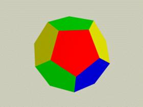
Figure 5. Dodecahedron
5.3. The “golden” algebraic equation
Denote a proportion (3) by x. Then, taking
into consideration that АВ = АС + СВ, the
proportion (3) can be written in the following form:
 ,
,
from where the following algebraic equation
follows:
x2 = x + 1 (4)
5.4. The golden mean
Eq. (4) has two real roots:
![]() and
and ![]() . (5)
. (5)
The positive root of the “golden” algebraic equation (4) is
called golden mean, golden ratio,
golden number or golden proportion. If we denote the golden mean by t, we
can write the following expression for the golden mean:
t = ![]() . (6)
. (6)
5.5. The remarkable properties of
the golden mean
tn = tn-1 + tn-2 = t´tn-1 (7)
 (8)
(8)
![]() (9)
(9)
5.6. Fibonacci and Lucas numbers
F(n)
= F(n-1) + F(n-2) (10)
F(0)
=0, F(1)
= 1 (11)
L(n)
= L(n-1) + L(n-2) (12)
L(0)
= 2; L(1) = 1 (13)
![]()
![]() (14)
(14)
Table 1
|
n |
0 |
1 |
2 |
3 |
4 |
5 |
6 |
7 |
8 |
9 |
10 |
|
F(n) |
0 |
1 |
1 |
2 |
3 |
5 |
8 |
13 |
21 |
34 |
55 |
|
F(-n) |
0 |
1 |
-1 |
2 |
-3 |
5 |
-8 |
13 |
-21 |
34 |
-55 |
|
L(n) |
2 |
1 |
3 |
4 |
7 |
11 |
18 |
29 |
47 |
76 |
123 |
|
L(-n) |
2 |
-1 |
3 |
-4 |
7 |
-11 |
18 |
-29 |
47 |
-76 |
123 |
As follows from
Table 1, the terms of the “extended” series F(n) and L(n) have a number of wonderful
mathematical properties
5.7. Cassini formula
In 17th century the
famous French astronomer Giovanni Domenico Cassini
(1625-1712) derived the most important identity for the Fibonacci numbers:
![]() (15)
(15)
5.8. Binet formulas for Fibonacci
and Lucas numbers
 (16)
(16)
 (17)
(17)
where the discrete variable n takes
its values from the set: 0, ±1, ±2, ±3,
6. The generalized Fibonacci
p-numbers and the generalized golden p-sections (Stakhov)
6.1. The generalized Fibonacci
p-numbers
In the second half of 20th century many Great mathematicians (Martin Gardner [5], George Polya [10], Alred Renyi [16] and others) independently one from other discovered the connection of the Fibonacci numbers with Pascal triangle and binomial coefficients. In the beginning of 70th years of 20th century Alexey Stakhov in his DrSci dissertation (1972) [12] and then in the book [13] introduced the so-called generalized Fibonacci p-numbers given by the following recursive relation:
Fp(n) = Fp(n-1)+Fp(n-p-1) for n>p+1 (18)
Fp(0) = 0, Fp(1) = Fp(2) = ... = Fp(p) = 1 (19)
where p=0, 1, 2, 3, … and n=0, ±1, ±2, ±3, …
They can be represented by binomial coefficients as follows [13]:
![]() (20)
(20)
Table 2. The
“extended” Fibonacci р-numbers
|
n |
8 |
7 |
6 |
5 |
4 |
3 |
2 |
1 |
0 |
-1 |
-2 |
-3 |
-4 |
-5 |
-6 |
-7 |
-8 |
-9 |
|
F1(n) |
21 |
13 |
8 |
5 |
3 |
2 |
1 |
1 |
0 |
1 |
-1 |
2 |
-3 |
5 |
-8 |
13 |
-21 |
34 |
|
F2(n) |
9 |
6 |
4 |
3 |
2 |
1 |
1 |
1 |
0 |
0 |
1 |
0 |
-1 |
1 |
1 |
-2 |
0 |
2 |
|
F3(n) |
5 |
4 |
3 |
2 |
1 |
1 |
1 |
1 |
0 |
0 |
0 |
1 |
0 |
0 |
-1 |
1 |
0 |
1 |
|
F4(n) |
4 |
3 |
2 |
1 |
1 |
1 |
1 |
1 |
0 |
0 |
0 |
0 |
1 |
0 |
0 |
0 |
-1 |
1 |
|
F5(n) |
3 |
2 |
1 |
1 |
1 |
1 |
1 |
1 |
0 |
0 |
0 |
0 |
0 |
1 |
0 |
0 |
0 |
-1 |
6.2. The generalized “golden” equations
(Stakhov)
If we take a ratio of the two adjacent Fibonacci p-numbers Fp(n)/Fp(n-1) and aim the number n for infinity, we will come to the generalized “golden” algebraic equation:
xp+1 = xp + 1. (21)
A set of the positive roots tp of the generalized “golden” equation are called the generalized golden p-proportions [13]. For p >0 they are a new class of irrational numbers, which express new, unknown until now properties of Pascal triangle. The generalized golden p-proportions possess the following remarkable property:
![]() (22)
(22)
6.3. A generalization of the
golden section (Stakhov)
Alexey Stakhov generalized the division in the extreme and mean ratio (the golden section) as follows [13]. Let us give the integer р=0, 1, 2, 3, ... and divide a line segment AВ with a point C in the following proportion (Fig. 6):
![]() (23)
(23)

Figure 6. The golden p-sections (p = 0, 1, 2, 3, ...)
As is shown in [13],
a solution of the problem (23) is reduced to the search of a positive root of
the equation (21), that is, the division of a line segment in the ratio (23) is
equal to the golden р-proportion tp.
Consider now the
partial cases of the golden р-section (23). It is clear
that for the case р=0 the golden р-section
(23) is reduced to the classical “dichotomy” (Fig. 6-а), and for the case p = 1 to the
classical golden section (Fig. 6-б).
For the rest values р we have an infinite
number of some proportional divisions of the line segment in the ratio (23). In
particular, it is easy to prove that for the case р®¥ the golden р-proportion tр ®1.
6.4. The
Generalized Principle of the Golden Section (Stakhov)
If we divide all terms of the identity (22) by ![]() we will get the following
identity:
we will get the following
identity:
![]() . (24)
. (24)
By
using (22), (24), we can construct the following “dynamic” model of the “Unit”
decomposition according to the role of the golden р-proportion:
 (25)
(25)
The
main result of the above consideration is finding some general principle of the
“Unit” representation through the golden p-proportion [71]:
![]() , (26)
, (26)
where tp is the golden p-proportion,
pÎ{0, 1, 2, 3, …}.
It
is clear that this general principle includes in itself the “Dichotomy
Principle” (p=0):
1 = 20 = 2-1 + 2-2
+ 2-3 +… (27)
and the classical “golden section principle” (p=1):
1 = t0
= t-1 + t-3 + t-5
+… (28)
7. The generalized Binet
formulas for the Fibonacci and Lucas p-numbers
(Stakhov, Rozin)
7.1. The generalized Binet formulas for the
Fibonacci p-numbers
Alexey Stakhov and Boris Rozin derived in [75] the following general formula for the analytical representation of the Fibonacci p-numbers:
Fp (n) = k1(x1)n
+ k2(x2)n
+ … + kp+1(xр+1)n,
where x1, x2, …, xp+1
are the roots of the generalized “golden” algebraic equation (21) and k1, k2, … , kp+1
are constant coefficients, the solutions of the following system of the
algebraic equation:
Fp (0) = k1
+ k2 + … + kp+1= 0
Fp (1) = k1x1 + k2x2
+ ...+ kp+1xр+1=1
Fp (2) = k1(x1)2 + k2(x2)2 + … + kp+1(xр+1)3=1
......................................................................
Fp (р) = k1(x1)р
+ k2(x2)р
+ … + kp+1(xр+1)р=1
7.2. Binet formula
for the Fibonacci 2-numbers
F2(n) = ![]()
![]() +
+ ![]()
 +
+
+ ![]()
 (29)
(29)
where
![]()
It
seems incredible at first sight that the formula (29),
which is apparently a complicated combination of complex numbers with irrational coefficients,
actually gives the integer Fibonacci 2-series
Fp(n) for any integer n = 0,
±1, ±2, ±3,
7.3.
The generalized Binet formula for the
Lucas p-numbers
In [75] the following generalized Binet formula was introduced:
Lp (n) = (x1)n + (x2)n + … + (xр+1)n (31)
where x1, x2, …, xp+1 are the roots of the generalized “golden” equation (21).
For a given p=0, 1, 2, 3, … the formula (31) sets an infinite number of the recursive series given by the recursive formula:
Lp(n) = Lp(n-1)+Lp(n-p-1) for n>p+1; (32)
Lp(0) = p+1, Lp(1) = Lp(2) = ... = Lp(p) = 1 (33)
where n=0, ±1, ±2, ±3, …(Table 3)
Table 3. The “extended” Lucas p-numbers
|
n |
9 |
8 |
7 |
6 |
5 |
4 |
3 |
2 |
1 |
0 |
-1 |
-2 |
-3 |
-4 |
-5 |
-6 |
-7 |
-8 |
-9 |
|
L1(n) |
76 |
47 |
29 |
18 |
11 |
7 |
4 |
3 |
1 |
2 |
-1 |
3 |
-4 |
7 |
-11 |
18 |
-29 |
47 |
-76 |
|
L2(n) |
31 |
21 |
15 |
10 |
6 |
5 |
4 |
1 |
1 |
3 |
0 |
-2 |
3 |
2 |
-5 |
1 |
7 |
-6 |
-6 |
|
L3(n) |
19 |
13 |
8 |
7 |
6 |
5 |
1 |
1 |
1 |
4 |
0 |
0 |
-3 |
4 |
0 |
3 |
-7 |
4 |
-3 |
|
L4(n) |
10 |
9 |
8 |
7 |
6 |
1 |
1 |
1 |
1 |
5 |
0 |
0 |
0 |
-4 |
5 |
0 |
4 |
-9 |
5 |
8. A theory of the Fibonacci matrices
8.1. The Fibonacci Q-matrix (Verner
Hoggatt)
Verner Hoggat in the book [9] developed a theory of the Fibonacci Q-matrix:
![]() (34)
(34)
 (35)
(35)
Det Qn = F(n-1)F(n+1) – F2(n)= (-1)n. (36)
Table 4. Fibonacci Q-matrices
|
n |
0 |
1 |
2 |
3 |
4 |
5 |
6 |
7 |
|
Qn |
|
|
|
|
|
|
|
|
|
Q-n |
|
|
|
|
|
|
|
|
8.2. The generalized Fibonacci Qp-matrices
(Stakhov)
8.2.1. A definition of
the Qp-matrix
Alexey Stakhov had developed in [67] a theory of the Fibonacci Qp-matrix:
 (p=0, 1, 2, 3, …) (37)
8.2.2. The partial
cases of the Qp-matrix
Q0 = (1) ; ![]() ;
;  ;
;
 ;
;  .
.
Note that for the case p=1 the Qp-matrix (37) is reduced to classical Q-matrix (34). Note also that the Qp-matrices have exceptional properties. For example, the Qp-1-matrix (p=1, 2, 3, …) can be obtained from the Qp-matrix by means of crossing out the last column and the next to the last row in the latter. It means that each Qp-matrix as if includes in itself all preceding Qp-matrices and is contained into all the next Qp-matrices.
8.2.3. The n-th power
of the Qp-matrix
 (38)
(38)
8.2.4. Determinant of
the matrix ![]()
Det ![]() = (- 1)np. (39)
= (- 1)np. (39)
9. The generalized Fibonacci
and Lucas numbers of the order m and
Gazale formulas (Spinadel, Gazale, Kappraff, Tatarenko).
9.1. The generalized Fibonacci and Lucas numbers of the order m
Spinadel, Gazale, Kappraff and Tatarenko independently one from another developed in [35, 38, 43, 89] the following generalizations of the Fibonacci and Lucas recursive relations:
Fm(n) = mFm(n-1) + Fm(n-2) (40)
Fm(0) = 0, Fm(1) = 1, (41)
![]() (42)
(42)
Lm(0) = 2, Lm(0) = m (43)
where m is a positive real number, n = 0, ±1, ±2, ±3, ... .
Here we denote by Fm(n) the generalized Fibonacci numbers of the order m and by Lm(n) the generalized Lucas numbers of the order m. Note that for the case m=1 the recursive formulas (40) and (42) are reduced to the recursive formulas (10) and (12), respectively.
9.2. The generalized Cassini formula
![]() (44)
(44)
9.3.
The “golden” algebraic equation of the order
m
x2 – mx – 1 = 0 (45)
Here m is a positive real number. The roots of the “golden” algebraic equation of the order m:
![]()
![]() (46)
(46)
Note that for the case m=1
the equation (45) is reduced to the classical “golden” equation (4)
9.4. The
generalized golden mean of the order m
![]() (47)
(47)
![]() ;
; ![]() ;
; ![]()
![]()

Thus, the generalized golden mean of the order m given by (47) is a wide generalization
of the classical golden mean (6), which is a partial case of (47) for m=1. The formula (47) generates an
infinite number of the generalized golden means because every positive real
number m originates its own
generalized golden mean of the order m.
9.5. Gazale formulas for the generalized
Fibonacci and Lucas numbers of the order m
![]()
![]() (48)
(48)
where m is a positive real number, Fm is the generalized golden mean of the order m, n=0, ±1, ±2, ±3, …
Table 4. The generalized Fibonacci
sequences of the orders m=1, 2, 3, 4
|
m |
Fm |
-5 |
-4 |
-3 |
-2 |
-1 |
0 |
1 |
2 |
3 |
4 |
5 |
|
1 |
|
5 |
-3 |
2 |
-1 |
1 |
0 |
1 |
1 |
2 |
3 |
5 |
|
2 |
1+ |
29 |
-12 |
5 |
-2 |
1 |
0 |
1 |
2 |
5 |
12 |
29 |
|
3 |
|
109 |
-33 |
10 |
-3 |
1 |
0 |
1 |
3 |
10 |
33 |
109 |
|
4 |
|
305 |
-72 |
17 |
-4 |
1 |
0 |
1 |
4 |
17 |
72 |
305 |
Table 5. The generalized Lucas sequences of
the orders m=1, 2, 3, 4
|
m |
Fm |
-5 |
-4 |
-3 |
-2 |
-1 |
0 |
1 |
2 |
3 |
4 |
5 |
|
1 |
|
-11 |
7 |
-4 |
3 |
-1 |
2 |
1 |
3 |
4 |
7 |
11 |
|
2 |
1+ |
-82 |
34 |
-14 |
6 |
-2 |
2 |
2 |
6 |
14 |
34 |
82 |
|
3 |
|
-393 |
119 |
-36 |
11 |
-3 |
2 |
3 |
11 |
36 |
119 |
393 |
|
4 |
|
-1364 |
322 |
-76 |
18 |
-4 |
2 |
4 |
18 |
76 |
322 |
1364 |
Analysis of the Gazale formulas (48) shows that these formulas generates an infinite number of the recursive numerical sequences similar to Fibonacci and Lucas numbers because every positive real number m (the order of the sequence) generates its own sequence. Note that for the case p=2 Gazale formulas (48) generate the numerical sequences known as Pell numbers and Lucas-Pell numbers [38, 88, 84].
10. The Fibonacci Gm-matrices of the order m
Alexey Stakhov introduced in [84] the Fibonacci Gm-matrix:
![]() (49)
(49)
 (50)
(50)
where m is a positive real number, n=0, ±1, ±2, ±3, …
Note that the classical Fibonacci Q-matrix (34) is a partial case of the Fibonacci Gm-matrices (49) for the case m=1. Also the matrices (35) is a partial case of the matrices (50) for the case m=1.
It
is easy to prove the following properties of the matrices ![]() :
:
Det ![]() = Fm(n+1)´Fm(n-1) -
= Fm(n+1)´Fm(n-1) - ![]() = (-1)n. (51)
= (-1)n. (51)
![]() (52)
(52)
Table 6. A sequence of
the matrices 
|
n |
0 |
1 |
2 |
3 |
4 |
5 |
|
|
|
|
|
|
|
|
|
|
|
|
|
|
|
|
Table 7. A sequence of
the matrices 
|
n |
0 |
1 |
2 |
3 |
4 |
5 |
|
|
|
|
|
|
|
|
|
|
|
|
|
|
|
|
Note that the formulas (49), (50) generate an infinite
number of the generalized Fibonacci Q-matrices
of the order m because every positive
real number m originates its own generalized
Fibonacci matrix of the order m.
Part 3. Application of the “Harmony
Mathematics” to theoretical physics.
New hyperbolic models of Nature
11. The hyperbolic Fibonacci
and Lucas functions (Stakhov, Tkachenko, Rozin)
11.1. The hyperbolic Fibonacci
and Lucas functions (Stakhov and Tkachenko’s definition)
Alexey Stakhov and Ivan Tkachenko
introduced in [62] a new class of hyperbolic functions, hyperbolic Fibonacci and Lucas functions, based on analogy
hyperbolic functions with Binet formulas (16) and (17).
11.1.1. Hyperbolic
Fibonacci sine and cosine
![]() ;
; ![]() (53)
(53)
11.1.2. Hyperbolic
Lucas sine and cosine
![]() ;
; ![]() (54)
(54)
where ![]() (the golden mean).
(the golden mean).
11.1.3. Connections with
the Fibonacci and Lucas numbers
sF(k) = F(2k); cF(k)
= F(2k+1); sL(k) = L(2k+1); cL(k) = L(2k) (55)
11.1.4. Some
identities for the hyperbolic Fibonacci and Lucas functions
sF(x) + cF(x) = sF(x+1); sL(x) + cL(x) = cL(x+1) (56)
![]() (57)
(57)
![]() (58)
(58)
![]() (59)
(59)
![]() (60)
(60)
![]() (61)
(61)
![]() (62)
(62)
![]() (63)
(63)
11.2. The symmetric hyperbolic Fibonacci and Lucas
functions (Stakhov and Rozin’s definition)
Alexey Stakhov and Boris Rozin
developed in [70] the so-called symmetric
hyperbolic Fibonacci and Lucas functions.
11.2.1. Symmetric
hyperbolic Fibonacci sine and cosine
![]()
![]() (64)
(64)
11.2.2. Symmetric hyperbolic Lucas sine and cosine
![]()
![]() (65)
(65)
where ![]() (the golden ratio).
(the golden ratio).
11.2.3. Connection with the Fibonacci
and Lucas numbers
![]() ;
; ![]() (66)
(66)
11.2.4. The graphs of the symmetric hyperbolic Fibonacci sine and cosine
Figure 7. Symmetric hyperbolic Fibonacci
and Lucas functions
11.2.5. The recursive properties of the symmetric hyperbolic Fibonacci and
Lucas functions
Table 7. The identities for Fibonacci and
Lucas numbers and for the symmetric hyperbolic Fibonacci and Lucas functions
|
The identities for Fibonacci and Lucas numbers |
The identities for the symmetric
hyperbolic Fibonacci and Lucas functions |
|
|
F(n+2) = F(n+1)
+ F(n) |
sFs(x+2) = cFs(x+1) + sFs(x) |
cFs(x+2) = sFs(x+1) + cFs(x) |
|
F(n) = (-1) n-1 F(-n) |
sFs(x) = - sFs(-x) |
cFs(x) = cFs(-x) |
|
F(n+3) + F(n)
= 2F(n+2) |
sFs(x+3)+cFs(x) = 2cFs(x+2) |
cFs(x+3)+sFs(x)=2sFs(x+2) |
|
F(n+3) - F(n)
= 2F(n+1) |
sFs(x+3) - cFs(x) = 2sFs(x+1) |
cFs(x+3) - sFs(x) = 2cFs(x+1) |
|
F(n+6) – F(n)
= 4F(n+3) |
sFs(x+6) + sFs(x) = 4cFs(x+3) |
cFs(x+6)+cFs(x) = 4sFs(x+3) |
|
F2(n) 2 - F(n+1)F(n-1)
= (-1)n+1 |
[sFs(x)]2 - cFs(x+1) сFs(x-1) = -1 |
[cFs(x)]2 - sFs(x+1) sFs(x-1) = 1 |
|
F(2n+1) = F2(n+1)2 + F2(n) |
cFs(2x+1)=[cFs(n+1)]2 + [cFs(x)]2 |
cFs(2x+1)=[sFs(n+1)]2 + [sFs(x)]2 |
|
F(3n) = F3(n+1)3
+ F3(n)3 – - F3(n-1)3 |
sFs(3x) = [cFs(x+1)]3+[sFs(x)]3- -[cFs(x-1)]3 |
cFs(3x) =[sFs(x+1)]3+[cFs(x)]3- - [sFs(x-1)]3 |
|
L(n+2) = L(n+1)
+ L(n) |
sLs(x+2) = cLs(x+1) + sLs(x) |
cLs(x+2) = sLs(x+1) + cLs(x) |
|
L(n) = (-1) n L(-n) |
sLs(x) = - sLs(x) |
cLs(x) = cLs(-x) |
|
L2(n) - 2(-1)n = L(2n) |
[sLs(x)]2 + 2 = cLs(2x) |
[cLs(x))2 - 2 = cLs(2x) |
|
L(n)+L(n+3) = 2L(n+2) |
sLs(x) + cLs(x+3) = 2sLs(x+2) |
cLs(x) + sLs(x+3) = 2cLs(x+2) |
|
L(n+1) L(n-1) – L2(n) = –5(–1)n |
sLs(x+1) sLs(x-1) – [cLs(x)]2= -
5 |
cLs(x+1) cLs(x-1) – [sLs(x)]2= 5 |
|
F(n+3) – 2F(n)
= L(n) |
sFs(x+3) - 2cFs(x) = sLs(x) |
cFs(x+3) - 2sFs(x) = cLs(x) |
|
L(n-1)+ L(n+1)
= 5F(n) |
sLs(x-1) + sLs(x+1) = = 5sFs(x) |
cLs(x-1) + cLs(x+1) = 5cFs(x) |
|
L(n) + 5F(n) = 2L(n+1) |
sLs(x) +5cFs(x) = cLs(x+1) |
cLs(x) +5sFs(x) = sLs(x+1) |
|
L2(n+1)2 + L2(n) = 5F(2n+1) |
[sLs(x+1)]2 +
[sLs(x)]2 = = 5cFs(x) |
[cLs(x+1)]2 +
[cLs(x)]2 = 5cFs(x) |
It follows from Table 7 that every “discrete” identity for the Fibonacci and Lucas numbers has its analogy in the form of the corresponding “continuous” identity for the symmetrical hyperbolic Fibonacci and Lucas functions. This means that after the introduction of the hyperbolic Fibonacci and Lucas functions the “Fibonacci numbers theory” lost its original significance because it is replaced by more general theory, a “theory of the hyperbolic Fibonacci and Lucas functions”.
11.2.6. The
hyperbolic properties of the symmetric hyperbolic Fibonacci and Lucas functions
In addition to the recursive
properties (see Table 7), the symmetric hyperbolic Fibonacci and Lucas
functions possess “hyperbolic properties” similar to the well-known properties
of the classical hyperbolic functions:
cFs2(x) – sF2s(x) = 4/5 (67)
cLs2(x) – sF2s(x) = 4 (68)
Note that the identities (67), (68) are analogies
of the well-known property of the classical hyperbolic functions:
ch2(x) – sh2(x) = 1.
Also we can prove the following identities for
the symmetrical Fibonacci and Lucas functions:
![]() cFs(x+y) = cFs(x)cFs(y)
+ sFs(x)sFs(y) (69)
cFs(x+y) = cFs(x)cFs(y)
+ sFs(x)sFs(y) (69)
![]() cFs(x-y) = cFs(x)cFs(y)
- sFs(x)sFs(y) (70)
cFs(x-y) = cFs(x)cFs(y)
- sFs(x)sFs(y) (70)
2cLs(x±y) = cLs(x)cLs(y) ± sLs(x)sLs(y) (71)
![]() sFs(2x) = sFs(x)cFs(x) (72)
sFs(2x) = sFs(x)cFs(x) (72)
sLs(2x) = sLs(x)cLs(x) (73)
As is proved in [70], all identities (69)-(73) have their analogies in the form of the corresponding identities for the classical hyperbolic functions.
11.3. The hyperbolic Fibonacci and Lucas functions
of the order m (Stakhov)
Gazale formulas (48) are a source for the introduction of a
new class of the hyperbolic Fibonacci and Lucas functions [84].
11.3.1. Hyperbolic Fibonacci sine of the order m
 (74)
(74)
11.3.2. Hyperbolic Fibonacci cosine of the order m
 (75)
(75)
11.3.3. Hyperbolic Lucas sine of the order m
 (76)
(76)
11.3.4. Hyperbolic Lucas cosine of the order m
 (77)
(77)
where m is a positive
real number, Fm is the
generalized golden mean of the order m.
11.3.4. Hyperbolic Fibonacci and Lucas functions of
the order m=1


11.3.5. Hyperbolic Fibonacci and Lucas functions of
the order m=2
![]()
![]()
![]()
![]()
11.3.6. Hyperbolic Fibonacci and Lucas functions of
the order m=3


11.3.7. Recursive
properties
sFm (x+2) = mcFm (x+1) + sFm (x) сFm(x+2)
= msFm(x+1) + cFm(x)
[sFs(x)]2 - cFs(x+1) сFs(x-1)
= -1 [cFs(x)]2 - sFs(x+1) sFs(x-1)
= 1
11.3.8. Hyperbolic properties
[cFm(x)]2 - [sFm(x)]2 = ![]() [cLs(x)]2
- [sLs(x)]2 = 4
[cLs(x)]2
- [sLs(x)]2 = 4
![]() cFm(x+y) = cFm(x)cFm(y) + sFm(x)sFm(y)
cFm(x+y) = cFm(x)cFm(y) + sFm(x)sFm(y)
![]() cFm(x-y) = cFm(x)cFm(y) – sFm(x)sFm(y)
cFm(x-y) = cFm(x)cFm(y) – sFm(x)sFm(y)
![]() cFm(2x) = [cFm(x)]2 + [sFm(x)]2
2cLm(2x) = [cLm(x)]2 + [sLm(x)]2
cFm(2x) = [cFm(x)]2 + [sFm(x)]2
2cLm(2x) = [cLm(x)]2 + [sLm(x)]2
[cFm(x) ± sFm(x)]n =  [cFm(nx) ± sFm(nx)]
[cLm(x) ± sLm(x)]n
= 2n-1[cFm(nx) ± sFm(nx)]
11.3.9. Applications to theoretical physics
In
conclusion we can note that the hyperbolic Fibonacci and Lucas functions of the
order m given by (74)-(77) are a wide generalization of the symmetric
hyperbolic Fibonacci and Lucas functions introduced in [70]. They are based on
the Gazale formulas (48) and extend infinitely a number of new hyperbolic
models of Nature. It is difficult to imagine, that a number of new hyperbolic
functions is so much, how many exist real numbers! And all of them possess
unique recursive and hyperbolic properties similar to the properties of the
classical hyperbolic functions and the symmetric hyperbolic Fibonacci and Lucas
functions [72]. This
fact is of great importance for the development of the contemporary hyperbolic
geometry and theoretical physics. We can predict that the applications of the
hyperbolic functions (74)-(77) to Lobachevski’s hyperbolic geometry and
Minkovski’s geometry (hyperbolic interpretation of Einstein’s relativity
theory) can result in new fruitful results in this important area. The first
result for this area was
obtained recently by the Ukrainian researcher Oleg Bodnar who proved in [30,
45] that the “golden” hyperbolic functions underlie phyllotaxis geometry.
12. The “golden” matrices (Stakhov)
12.1. The “golden” matrices based on the
symmetric hyperbolic Fibonacci functions
Alexey Stakhov introduced in [79]
a new class of the square matrices called the “golden” matrices:
![]() (78)
(78)
 (79)
(79)
12.2. Determinants of the “golden” matrices
Det Q2x = cFs(2x+1)´cFs(2x-1) – [sFs(2x)]2 = 1 (80)
Det Q2x+1 = sFs(2x+2)´sFs(2x) – [cFs(2x+1)]2 = -1 (81)
Note that the “golden” matrices (78), (79) are a natural generalization of the matrix (35) for continuous domain. Also the formulas (80) and (81) are a generalization of the formula (36).
12.3. The “golden” matrices based on the
hyperbolic Fibonacci functions of the order m
Alexey Stakhov introduced in [84]
a new class of the “golden” matrices based on the hyperbolic Fibonacci
functions of the order m:
 (82)
(82)
 (83)
(83)
12.4. Determinants of the “golden” matrices of
the order m
Det ![]() = cFm(2x+1)´cFm(2x-1) – [sFm(2x)]2 = 1 (84)
= cFm(2x+1)´cFm(2x-1) – [sFm(2x)]2 = 1 (84)
Det ![]() = sFm(2x+2)´sFm(2x) – [cFm(2x+1)]2 = -1 (85)
= sFm(2x+2)´sFm(2x) – [cFm(2x+1)]2 = -1 (85)
Note the “golden” matrices (82) and (83) are a generalization of the matrices (78) and (79), which are partial cases of the matrices (82) and (83) for m=1. Also the formulas (84) and (85) are a generalization of the formulas (80) and (81), which are partial cases of the formulas (84) and (85) for m=1. It is important to note that a number of the matrices (82) and (83) is infinite because every positive real number m originates its own “golden” matrix of the kind (82) and (83).
Part 4. Application of the “Harmony
Mathematics” to measurement theory and number theory
As we mentioned in Part 1, there are two fundamental mathematical theories, number theory and measurement theory, which underlie historically the “classical mathematics” (see Fig.1). A number theory is named sometimes a “Tsarina of Mathematics” what emphasizes a fundamental role of number theory in mathematics. Below we will try to demonstrate how the “Harmony Mathematics” can influence on the development of these fundamental mathematical theories.
13. Algorithmic measurement theory (Stakhov)
13.1. Classical measurement theory
The classical measurement theory is based on the “continuity axioms” (Eudoxus-Archimedus’ axiom and Cantor’s axiom). Its main result [93] is a proof of the existence and uniqueness of the solution q of the basic measurement equality:
Q = qV, (86)
where V is a measurement unit, Q is
a measurable segment, q is any real
number named a result of measurement.
The idea of the proof of the measurement equality (86) consists in the following [93]. By using Eudoxus-Archimedus’ axiom and by following the certain rules called a measurement algorithm, we can form from the measurement unit V some sequence of the “contractible segments”, which are compared with the measurable segment Q. If we direct this process ad infinitum, then according to Cantor’s axiom for the given Q and V we always can find such “contactable segment”, which coincides with the measurable segment Q. It is important to note that it follows from Canto’s axiom that measurement is a process ending for infinite time (Cantor’s abstraction of actual infinity).
In 20th century Cantor’s abstraction of actual infinity was subjected to merciless criticism in the “constructive mathematics”, which uses in its axioms and theorems another concept of the “mathematical infinity”, potential infinity [108]. Thus, the development of 20th century mathematics demanded on a revision of mathematical measurement theory from the “constructive idea” [108]. The main purpose of the “constructive measurement theory” [13, 14] is searching the “optimal” measurement algorithms. This problem is solved in the “algorithmic measurement theory” [13, 14], which is a wide generalization of Bashet-Mendelleev’s problem [13], the first optimization problem in measurement theory.
13.2. The “Asymmetry Principle of Measurement”
As is known, a solution of Bashet-Mendelleev’s problem [13] is reduced to the “binary” measurement algorithm, which uses the "binary" standard weights 2n-1, 2n-2 , ..., 20 for measurement. Analysis of the “binary” algorithm resulted in the discovery of some general property of measurement called the “Asymmetry Principle of Measurement” [13, 54].
Figure 9. Asymmetry Principle of Measurement
We will analyze the “binary” measurement algorithm by means of the use of the balance model (Fig.9). This analysis allows to find a measurement property of general character for any thinkable measurement, based on the comparison of the measurable weight Q with the standard weights.
Consider now the weighing process of the weight Q on the balance, by using some “binary” standard weights. On the first step of the “binary” algorithm the largest standard weight 2n-1 is placed on the free cup of the balance (Fig. 9-a), which compares the weight Q with the largest standard weight 2n-1. After the comparison we can get two situations: 2n-1 < Q (Fig. 9-a) and 2n-1 ³ Q (Fig. 9-b). In the first case (Fig. 9-a) the second step is to add the next large standard weight 2n-2 on the free cup of the balance. In the second case (Fig.9-b) the “weigher” should perform two operations, that is, to remove the previous standard weight 2n-1 from the free cup of the balance (Fig. 9-b), after that the balance should return to the initial position (Fig. 9-c). After returning the balance to the initial position, the next standard weight 2n-2 is placed on the free cup of the balance (Fig. 9-c).
One can readily see that the both considered cases differ by their “complexity”. Really, for the first case, the “weigher” have to fulfill only one operation to add the next standard weight 2n-2 on the free cup of the balance. For the second case, the “weigher’s” actions are determined by two factors. First of all, he has to remove the previous standard weight 2n-1 from the free cup of the balance and after that he has to take into consideration a time necessary for returning back the balance to the initial position. The discovered property of measurement was called the Asymmetry Principle of Measurement [13, 54].
13.3. The unexpected results of the algorithmic
measurement theory
The
algorithmic measurement theory based on the “Asymmetry Principle of
Measurement” are presented in author’s books [13,14]. For English readers we
can recommend Stakhov’s article [59]. The investigation of the optimal measurement algorithms resulted in the discovery
of new, unknown measurement
algorithms. They are described [13,14, 59] by very complex recursive
relation Fp(n, k),
which for a given p (p=0, 1, 2, 3, ...) depends on two discrete
variables n and k (n=0, 1, 2, 3, ...; k=0, 1, 2, 3,
...). Note that p is a discrete time necessary for returning the balance
from the position in Fig. 9-b to the position in Fig. 9-c after removing the
standard weight from the “free” cup of the balance; n is a number of
steps of the algorithm and k is a number of balances participated in
measurement. The recursive relation Fp(n,
k) gives a number of the quantized levels provided by the optimal (n,k)-measurement algorithms.
Table 8. The unexpected results of the algorithmic measurement theory
|
|
p = 0 |
|
0 £ p £ ¥ |
|
p = ¥ |
|
|
k ³ 1 |
|
|
Fp(n, k) |
|
|
Binomial Coeff. |
|
|
|
|
|
|
|
|
|
k = 1 |
2n |
|
Fp(n) = Fp(n-1) + Fp(n-p-1) |
|
n+1 |
|
|
|
Binary sequence |
|
Fibonacci p-numbers |
|
Natural numbers |
|

It is
proved in [13,14, 59] that for different p,
n and k the recursive formula Fp(n,
k) originates many well-known combinatorial formulas, in particular, the
formula (k+1)n for p=0, the formula 2n
for p=0 and k=1, the formula for the binomial coefficients ![]() for p = ¥, the
formula n+1 given natural numbers for p
= ¥
and k=1 and, ultimately, the
recursive formula for the Fibonacci p-numbers
for k=1.
for p = ¥, the
formula n+1 given natural numbers for p
= ¥
and k=1 and, ultimately, the
recursive formula for the Fibonacci p-numbers
for k=1.
The new
measurement algorithms include all classical measurement algorithms, in
particular, the “binary” algorithm. There is an isomorphism between measurement
algorithms and positional number systems. This idea gives us a right to put
forward the hypothesis that the algorithmic measurement theory is a source of a new theory of positional number systems.
14. Number systems
with irrational radices and a new definition of real numbers
14.1. Geometric
definition of real number
We can
develop the so-called “constructive approach” to the definition of “real
number”. According to this approach [108] the real number A is some mathematical object, which can be represented in binary
system as follows:
![]() (87)
(87)
where A
is any real number, ai
is binary numeral (0 or 1) of the i-th digit, i = 0, ±1, ±2,
±3, 2i is the “weight” of the i-th digit, the
number 2 is the base of numeral system (87).
The definition of the real number A given by (87) has the following geometric interpretation. Consider
now an infinite set of the “binary” line segments of the length 2n, that is,
B = {2n} (88)
where n = 0, ±1, ±2,
±3, …. Then all real numbers can
be represented by the sum (87), which consists of the “binary” segments taken
from (88).
Note that a number of the terms, included to the sum (87)
is always finite but potentially unlimited, that is, the definition (87) is a
brilliant example of the potential infinity concept used in the “constructive”
mathematics [108].
Clearly, that the definition (87) gives on the numerical
axis only a part of real numbers, which can be represented by the sum (87). We
will name such numbers constructive real
numbers. All other real numbers, which cannot be represented by the sum (87),
are non-constructive real numbers.
What numbers can be referred to the “non-constructive”
numbers within the framework of the definition (87)? Clearly, that all
irrational numbers, in particular, the main mathematical constants p and е, the
number![]() , the golden mean are referred to the “non-constructive” numbers.
But within the framework of the definition (87) some “rational” numbers (for
example, 2/3, 3/7, etc.), which cannot be represented by the final sum (87),
are referred to the “non-constructive” numbers.
, the golden mean are referred to the “non-constructive” numbers.
But within the framework of the definition (87) some “rational” numbers (for
example, 2/3, 3/7, etc.), which cannot be represented by the final sum (87),
are referred to the “non-constructive” numbers.
Note that though the definition (87) considerably limits
the set of real numbers, this fact does not belittle his significance from the
“practical”, computing point of view. It is easy to prove, that any
“non-constructive” real number can be represented by (87) approximately, and
the approximation error D
will decrease in the process of increasing the terms in (87), however D¹0 for all “non-constructive” real numbers. Really, in
modern computers we use only the “constructive” numbers given by (87), however
we do not have any problem with the “non-constructive” numbers, because they
can be represented in the form (87) with the approximation error that strives
to 0 potentially.
14.2. Bergman’s number system
We can use the golden mean t for a new constructive definition of real number. Consider now an infinite set of the “golden” line segments
of the length tn, that is,
B = {tn} (88)
where n = 0, ±1, ±2,
±3, ….
Then we can use the set (88) for the
following constructive definition of real numbers:
![]() , (89)
, (89)
where A
is any real number, ai
is binary numeral (0 or 1) of the i-th digit, i = 0, ±1, ±2,
±3, ti is the “weight” of the i-th digit, t (the golden mean) is the base of numeral system (89).
Note
that the numeral system (89) was introduced in 1957 by
the young American mathematician George Bergman [85]. The most surprising is the fact that George Bergman made his
mathematical discovery in the age of 12 years!
14.3. Codes of the golden
p-proportion
Also we
can use the golden p-proportion tp for more general
definition of real numbers. Consider an infinite set of the line segments based
on the golden p-proportions:
B = {![]() }, (90)
}, (90)
where n = 0, ±1, ±2,
±3, ….
Then we can use the set (90) for the construction of the
following positional numeral system:
![]() , (91)
, (91)
where A
is any real number, ai
is binary numeral (0 or 1) of the i-th digit, i = 0, ±1, ±2,
±3, ![]() is the “weight”
of the i-th digit, tp (the golden p-proportion)
is the base of numeral system (91).
is the “weight”
of the i-th digit, tp (the golden p-proportion)
is the base of numeral system (91).
We will name the sum (91) the code of the golden p-proportion.
Note that for p=0
the code of the golden p-proportion
(91) is reduced to the classical “binary” system (87) and
for p=1 to Bergman’s system (89).
Because all radices tp for p>0
are irrational numbers, this means that the sum (91) gives more general class
of numeral systems with irrational radices than Bergman’s system (89).
The numeral systems (91) were
introduced by Alexey Stakhov in 1980 in the article [56] and later in the book
[17].
Possibly the numeral systems (89)
and (91) are the most important
mathematical discovery in the field of numeral systems after the discovery
of positional principle of number representation (Babylon, 2000 B.C.) and
decimal system (India, 5th century).
14.4. Z-property and
D-property of natural numbers
Bergman’s
system (89) and codes of the golden p-proportion
(91) are a source of new number-theoretical results. The Z-property of natural numbers is one of such number-theoretical
results. This property is based on the following very simple reasoning.
Consider now the
representation of the natural number N
in Bergman’s system (89):
![]() (92)
(92)
The
representation of the natural number N
in the form (92) is called the t-code of natural number N.
It is proved in [69] that the sum (92) is finite for arbitrary
natural number N. This means that
arbitrary natural number N can be
represented in the form of finite sum of the golden mean power!
If we consider the well-known
formula
![]() (93)
(93)
and then substitute (93) into (92) we can represent the sum (92) as follows:
N = ![]() (A + B
(A + B![]() ), (94)
), (94)
where
A = ![]() ; (95)
; (95)
B = ![]() . (96)
. (96)
Note that all binary numerals in the
sums (95) and (96) coincide with the corresponding binary numerals of the t-code of natural number N
given by (92).
Represent now the formula (94) in the following form:
2N = A + B![]() . (97)
. (97)
Note that
the formula (97) has general character and is valid for arbitrary natural
number N.
Analyze now the formula (97). It is
clear that the number 2N, which stands
in the left-hand part of the formula (97), is an even number always. The right-hand
part of the formula (97) is the sum of the number A and the product of the number B
by the irrational number![]() . But according to (95) and (96) the numbers A and B are integers always because the Fibonacci and Lucas numbers are
integers. Then it follows from (94) that for the given natural number N the even number 2N is equal identically to the sum of the integer A and the product of the integer B by the irrational number
. But according to (95) and (96) the numbers A and B are integers always because the Fibonacci and Lucas numbers are
integers. Then it follows from (94) that for the given natural number N the even number 2N is equal identically to the sum of the integer A and the product of the integer B by the irrational number![]() . And this unusual statement is valid for arbitrary natural
number N! Then we can ask the
question: for what condition the identity (94) could be valid in general case?
The answer to this question is very simple: the identity (94) can be valid for arbitrary
natural number N only if the sum (96)
is equal to 0 (“zero”) identically and the sum (95) is equal to the double
number of N, that is
. And this unusual statement is valid for arbitrary natural
number N! Then we can ask the
question: for what condition the identity (94) could be valid in general case?
The answer to this question is very simple: the identity (94) can be valid for arbitrary
natural number N only if the sum (96)
is equal to 0 (“zero”) identically and the sum (95) is equal to the double
number of N, that is
B = ![]() = 0 (98)
= 0 (98)
A = ![]() = 2N (99)
= 2N (99)
The outcomes (98) and (99) have a
general character and are valid for all natural numbers, that is, our simple
reasoning’s resulted in new properties of natural numbers called Z-property and D-property of natural numbers [69].
Z-property. If we represent arbitrary natural number N in Bergman’s system (92) and then substitute
every power of the golden ratio ti in the sum (92) by
the Fibonacci number F(i), where the index i takes its values from the set {0, ±1, ±2, ±3, …}, then the sum, which
arises as a result of such substitution, is equal to 0 identically
independently on the initial natural number N.
D-property. If we represent arbitrary natural number N in Bergman’s system (92) and then substitute
every power of the golden ratio ti in the sum (92) by
the Lucas number L(i), where the index i takes its values from the set {0, ±1, ±2, ±3, …}, then the sum, which
arises as a result of such substitution, is equal to 2N identically independently on the initial natural number N.
Thus, we can see from this consideration that the “Harmony
Mathematics” can influence on the development of the fundamental theories of
mathematics, measurement theory and number theory.
Part 5. Applications of the “Harmony
Mathematics” to computer science
15. Fibonacci arithmetic (Stakhov)
15.1. Zeckendorf’s representation
In 1939 the Belgian amateur of mathematics Edurdo Zeckendorf introduced the following positional representation called Zeckendorf’s representation:
N = an F(n)
+ an-1 F(n-1) + ... + ai F(i)
+ ... + a1F(1) (100)
where ai is a binary numeral (0 or 1) of the i-th digit of the code representation (100); F(i) is the “weight” of the i-th digit of the code representation (100).
15.2. Fibonacci p-codes (Stakhov)
Fibonacci’s measurement algorithms [13] originate the following positional representation called the Fibonacci p-code:
N = anFp(n) + an-1Fp(n-1) + ... + aiFp(i)
+ ... + a1Fp(1) (101)
where p=0, 1, 2, 3, …; ai is a binary numeral (0 or 1) of the i-th digit of the code representation (101); Fp(i) is the “weight” of the i-th digit of the code representation (101).
Note that for p=0 the Fibonacci p-code (101) is reduced to the “binary” representation
N = an2n-1 + an-12n-2 + ... + ai2i-1 + ... + a120 ,
for p=1 to Zeckendorf’s representation (100) and for p=¥ to the so-called “unitary
code” ![]()
15.3. A concept of Fibonacci computer
The first attempt to design computer and measurement systems based on Fibonacci representations (100) and (101) was undertaken in the past Soviet Union during 70-80th years of the 20th century. 65 patents on the Soviet computer inventions given by the State Patenting Offices of USA, Japan, England, Germany, France, Canada and other countries are confirmation of the Soviet science priority in this important computer field. Scientific researches and engineering developments [23] did demonstrate a high effectiveness of the Fibonacci codes (100) and (101) and following from them Fibonacci arithmetic for designing self-correcting analog-to-digit and digit-to-analog converters and noise-tolerant processors. Also the Fibonacci p-codes (101) originated new super-fast transformations for digital signal processing [109, 110].
16.Ternary mirror-symmetrical arithmetic (Stakhov)
16.1. Brousentsov’s ternary principle of designing
computers
It is well known that modern
computers are based on the famous “John von Neumann “Binary” Principle”: binary
system, binary (Boolean) logic, binary memory element (“flip-flop”). However, at the dawn of the computer
era the original computer project (the ternary “Setun” computer) [111] was
designed in 1958 in
16.2. The ternary mirror-symmetric representation
Alexey Stakhov developed in [68] the original ternary representation of natural numbers based on the golden mean. This representation is based on the following properties of the golden mean t:
2t2k = t2(k+1) - t2k + t2(k-1) (102)
3t2k = t2(k+1) + 0 + t2(k-1) (103)
4t2k = t2(k+1) + t2k + t2(k-1) (104)
where k = 0, ±1, ±2, ±3, ... .
For the case k=0 we can write the identities (102)-(104) as follows:
2 = t2 - 1 + t -2 (105)
3 = t2 + 0 + t -2 (106)
4 = t2 + 1 + t -2 (107)
By using (105)-(107), we can represent all natural numbers by the even powers of the golden mean. For example, by representing the number 5 in the form 5=3+2 and by using (105) and (106), we can write:
5=3+2 = 2t2 - 1 + 2t -2 (108)
However, by using (102), we can represent 2t2 (k=1) and 2t -2 (k=-1) as follows:
2t2 = t4 - t2 + t0 (109)
2t -2 = t0 - t- -2 + t -4 (110)
By using (109) and (110), we can represent the sum (108) as follows:
5 = t4 - t2 + 1 - t- -2 + t -4 (111)
Then, we can represent the number 6 as follows:
6=5+1 = t4 - t2 + (1+1) - t- -2 + t -4 = t4 - t2 + 2 - t- -2 + t -4 (112)
By using (105), we can represent the sum (112) as follows:
6 = t4 - 1 + t -4 (113)
It is clear that the numbers 7 and 8 can be represented as follows:
7 = 6+1 = t4 + t -4 (114)
8 = 7+1 = t4 + 1 + t -4 (115)
And now we can use the ternary numerals {1, 0,`1} for abridged representation of the sums:
1 = 0 1, 0
2 = 1`1, 1
3 = 1 0, 1
4 = 1 1,1
5 = 1`1 1,`1 1
6 = 1 0`1, 0 1
7 = 1 0 0, 0 1
8 = 1 0 1, 0 1
Note that by using the rule of the “ternary inversion
1 ®`1; 0 ®0; `1®1, (116)
we can transform very easy positive integer number to the negative integer number, for example:
-1 = 0`1, 0
-2 = `1 1,`1
- 3 = `1 0,`1
- 4 = `1`1,`1
and so on.
It is proved in [66] that arbitrary integer N can be represented as follows:
![]() , (117)
, (117)
where ci is
the ternary numeral (1, 0,`1) of the ith digit; t2i
is the “weight” of the ith digit; ![]() is the base or radix
of the numeral system (116), i = 0, ±1,
±2, ±3, … .
is the base or radix
of the numeral system (116), i = 0, ±1,
±2, ±3, … .
Thus, a new positional representation of integers (117) is the main outcome of our consideration. This positional numeral system has the following peculiarities:
(1) The numeral system (117) is ternary because the ternary numerals (1, 0,`1) are used for number representation.
(2)
The irrational number ![]() (a square of the golden mean) is a radix of numeral system
(117), that is, the numeral system (117) is a number system with irrational
radix.
(a square of the golden mean) is a radix of numeral system
(117), that is, the numeral system (117) is a number system with irrational
radix.
(3) All integers (positive and negative) can be represented in the numeral system (117) and there is a simple rule (116) to transform positive number into negative one and conversely.
(4) All ternary representations of integers in the numeral system (117) possess the property of the "mirror symmetry": the left-hand part of these representations is mirror-symmetrical to its right-hand part relatively to the 0-th digit. Based on this fundamental property, the "ternary numeral system" given by (117) is called ternary mirror-symmetrical numeral system [68].
16.3. Ternary mirror-symmetrical arithmetic
16.4.1. Ternary mirror-symmetrical summation and subtraction
The identities (102)-(104) underlie ternary mirror-symmetrical summation (see Table 9).
Table 9. Mirror-symmetrical summation
|
bk ak |
|
0 |
1 |
|
|
|
|
0 |
|
0 |
|
0 |
1 |
|
1 |
0 |
1 |
1 |
The main peculiarity of Table 9 consists in the summation rule of two ternary units with equal signs, that is,
We can see that at the mirror-symmetrical summation of the ternary units with the same sign the intermediate sum sk with the opposite sign and the carry-over ck with the same sign appear. However, the carry-over from the kth digit spreads simultaneously to the next two digits, namely to the next left-hand, that is, (k+1)th digit, and to the next right-hand, that is, (k - 1)th digit. The main unexpected property of the mirror-symmetric summation of multi-digit numbers consists in the fact that the summation results are represented always in the mirror-symmetrical form. This means that we can check results of mirror-symmetrical summation.
The mirror-symmetrical subtraction is reduced to the mirror-symmetrical summation, if we represent the remainder in the following form:
N1 - N2 = N1 + (- N2). (118)
16.4.1. Ternary mirror-symmetrical multiplication and division
The following trivial identity for the golden mean powers underlies the mirror-symmetric multiplication:
t2n ´ t2m = t2(n+m) . (119)
The rule of the ternary mirror-symmetric multiplication is given in Table 10.
Table
10. Mirror-symmetric multiplication
|
|
|
0 |
1 |
|
|
1 |
0 |
|
|
0 |
0 |
0 |
0 |
|
1 |
|
1 |
1 |
The ternary mirror-symmetric multiplication is performed in the “direct” code. The general algorithm of the multiplication of two multi-digit mirror-symmetrical numbers is reduced to the formation of the partial products in accordance with Table 9 and their summation in accordance with the rule of the mirror-symmetric summation.
As example we will consider the multiplication of the negative mirror-symmetrical number
- 6 = `1 0 1, 0`1 by the positive mirror-symmetrical number 2 = 1`1, 1:

The multiplication result is formed as the sum of three partial products. The first partial product `1 0, 1 0`1 is the result of multiplication of the mirror-symmetrical multiplier - 6 = `1 0 1, 0`1 by the lowest positive unit of the mirror-symmetric multiplier 2 =1`1,1, the second partial product 1 0`1, 0 1 is the result of the multiplication of the same number - 6 = `1 0 1, 0`1 by the middle negative unit of the number 2=1`1, 1, and, finely, the third partial product `1 0 1, 0`1 is the result of the multiplication of the same number - 6 = `1 0 1, 0`1 by the higher positive unit of the number 2 = 1`1, 1.
Note that the product -12 =`1 1 0`1, 0`1`1 is represented in the mirror-symmetrical form! Because its higher digit is a negative unit `1 , it follows from here that the product is a negative mirror-symmetrical number.
The division of the ternary mirror-symmetrical numbers is similar to the division in the classical ternary-symmetrical numeral system [111].
Thus, we developed in [68] interesting computer arithmetic. Its main peculiarity consists in the fact that all arithmetical operations are carried out in the “direct” code and can be checked according to the mirror-symmetric property. This means that this arithmetic can be used for designing reliable computers.
17. A new theory of error-correcting codes based on the Fibonacci
matrices (Stakhov)
17.1. General principles of designing error-correcting
codes
The main idea of error-correcting codes (Hamming code, Reed-Solomon code, Reed-Muller code, Golay code, turbo code and so on) consists in the following [112]. Let the initial code combination consists of n data bits. We add to the initial code combination m error-correction bits and then form k-digit code combination of error-correcting code, or (k,n)-code, where k = n+m. The error-correction bits are formed from the data bits as the sums by module 2 of the certain groups of the data bits. It is clear that there are 2n different k-digit binary combinations of the error-correcting code a1, a2, a3, …, a2n. These binary combinations are called allowed binary combination. However, in general by using k digits, we can form 2k = 2n+m different binary combinations. We will divide them into two non-crossing groups, the 2n allowed binary combinations and the 2k - 2n prohibited binary combinations. We can send to a channel one of 2n allowed binary combination. Under influence of noise in the channel, this binary combination can turn into one of 2k possible binary combinations. This means that there are N= 2n´2k possible transitions because every of the 2n allowed combinations can turn into one of the 2k possible combinations. A principle of the error detection is based on the fact that the allowed binary combination turns into the prohibited binary combination. The number of the detectable transitions is equal Nd = 2n´(2k-2n). If we take a ratio Nd/N we will obtain the first numerical characteristic of the error-correcting code, called coefficient of potential detecting ability:
![]() (120)
(120)
where m is a number of error-correction bits.
A principle of error correction consists in the following. All 2k - 2n prohibited binary combinations are divided into the 2n non-crossing sets M1, M2, M3, …, M2n, where 2n is the number of the allowed binary combination. Every allowed binary combination is attributed to one of the 2n sets: a1®M1, a2®M2, a3®M3, …, a2n®M2n. A principle of error correction consists in the following. If we receive the prohibited code combination, which belongs to the set Mi, we assume that the allowed binary combination ai was transmitted. This means that we correct all erroneous binary combinations of the set Mi, if they are formed from the allowed binary combinations ai. In opposite case, a correction of the error is performed incorrectly. It is clear that the number of the correctable erroneous transitions Nc is equal to the number of all prohibited combinations, that is, Nc = 2k-2n.
A coefficient of potential correcting ability is calculated as a ratio of all correctable erroneous transitions Nc to all detectable transitions, that is,
![]() (121)
(121)
where n is a number of data bits in the code combination of error-correcting code.
The coefficients (120) and (121) characterize potential ability of error-correcting code to detect and correct errors.
An absolute redundancy of the error-correcting code is determined by the number m of error-correction bits. A relative redundancy of the error-correcting code is determined by the ratio
![]() (122)
(122)
Note that this reasoning
is valid for all error-correcting codes, that is, the estimations (120)- (122)
has a fundamental character for all error-correcting (k, n)-codes.
For example, the Hamming (15,11)-code is characterized by the following numerical parameters: k=15, n=11, m=4. This means that Hamming (15,11)-code has a relative redundancy R=0,27 (27%). Besides, the coefficient of potential detecting ability (120) for this code is equal Sd = 0.9375 (93,75%), this code guarantees the detection of all single and double errors in the code combination and the correction of all single errors in the 15-digit code combination of the Hamming code.
The formula (120) shows that the coefficient of potential detecting ability of the error-correcting code increases very quickly and aims for 100% as the number m increases. And this fact confirms a high effectiveness of the error-correcting codes to detect errors. However, the formula (121) shows that the coefficient of potential correcting ability diminishes potentially as the number n increases. For example, the Hamming (15,11)-code allows to detect 211´(215 - 211) = 62 914 560 erroneous transitions; at that the code can correct only 215 - 211 = 30720 erroneous transitions, that is, the code can correct only 30720 erroneous transitions among 62 914 560 erroneous transitions. Their ratio given by (121) Sc= 0, 0004882 (0, 04882%) characterizes a potential correcting ability of the Hamming (15,11)-code .
This simple analysis of general principles of designing error-correcting codes allows point out a number of essential disadvantages of the existing error-correcting codes [112]:
(1) A very low potential correcting ability, which is determined by the formula (121).
(2) One more fundamental disadvantage of all known error-correcting codes is the fact that the very small information items, bits and their combinations, are the objects of detection and correction.
We can ask two questions:
(1) Whether is it possible to create the theory of error-correcting codes, in which the larger information elements, for example, numbers or even files, were an object of detection and correction?
(2) How to increase a correcting ability of error-correcting codes?
We can find the answer to these questions in the book [37] and the article [78].
17.2. Fibonacci encoding/decoding
method
Let us consider the Fibonacci
encoding/decoding method introduced in [37, 78]. Let us represent the initial
information in the form of the square (p+1)´(p+1)-matrix M. Let us choose the “direct” Fibonacci Qp-matrix ![]() and “inverse”
Fibonacci Qp-matrix
and “inverse”
Fibonacci Qp-matrix ![]() as encoding and
decoding matrices, respectively. Then, we can construct the following Fibonacci
encoding/decoding method (see Table 11).
as encoding and
decoding matrices, respectively. Then, we can construct the following Fibonacci
encoding/decoding method (see Table 11).
Table 11. Fibonacci encoding/decoding method
|
Encoding |
Decoding |
|
M´ |
E´ |
It follows from Table 11 that for a given p (p=0, 1, 2, 3, …) the Fibonacci encoding
consists in multiplication of the initial (p+1)´(p+1)-matrix M by the encoding matrix ![]() given by (38). The
code matrix E is a result of such matrix multiplication. Then the
Fibonacci decoding consists in multiplication of the code matrix E by
the “inverse” matrix
given by (38). The
code matrix E is a result of such matrix multiplication. Then the
Fibonacci decoding consists in multiplication of the code matrix E by
the “inverse” matrix![]() .
.
17.3. The main checking identities
As is proved in [78], there is the following surprising identity connecting the determinants of the code matrix E with the determinant of the data matrix M:
Det E = Det M ´(-1)pn (119)
where p=1, 2, 3, …, n = 0, ±1, ±2, ±3, …
The
identity (119) is the main checking relation of the code matrix used for detection and correction errors in
the code matrix.
The simplest variant of the Fibonacci encoding/decoding is to use the Fibonacci Q-matrix (35) as the encoding matrix. For this case the data matrix M has the following form:
 (120)
(120)
where m1, m2, m3, m4 are some positive integers.
The code matrix E has the following form:
![]() , (121)
, (121)
where the elements e1, e2, e3, e4 are equal:
e1 = Fn+1 m1 + Fn m2 (122)
e2 = Fn m1 + Fn-1 m2 (123)
e3 = Fn+1 m3 + Fn m4 (124)
e4 = Fn m3 + Fn-1 m4 (125)
The main checking relation (119) for this case (p=1) has the following form:
Det E = - Det M´(-1)n (126)
Also it is proved in [78] the following approximate ratios, which connect the elements of the code matrix E:
e1 » te2 ; (126)
e3 » te4 , (127)
where ![]() is the golden mean.
is the golden mean.
Note that the elements
of the code matrix E given (122)-(125)
are integers always.
17.4. A notion of errors
A notion of “errors” in a new
coding theory differs from similar notion in the classical theory of
error-correcting code [122]. As is known, the “single” error is a transition of
bit in the opposite state (1®0 or 0®1). In our coding theory the “single” error is a
transition of any element of the code matrix E into “erroneous” state. If, for example, the “valid” element e1 is decimal numeral equal to 5, then the “single” error in the element
e1 is its transition into one of decimal numbers 0-4 or 6-9. It is clear that there are four (![]() ) variants of the “single” errors in the code matrix (121):
) variants of the “single” errors in the code matrix (121):
 ;
;  ;
;  ;
;  , (128)
where x, y, z, v are the
“erroneous elements” of the code matrix E.
Consider now the case of the “double” errors. There
are six (![]() ) variants of the “double errors”:
) variants of the “double errors”:
 ;
;  ;
;  ;
;  ;
;  ;
; ![]() . (129)
. (129)
It is clear that there are
four (![]() ) variants of the “triple” errors:
) variants of the “triple” errors:
 ;
;  ;
; ![]() ;
; ![]() . (130)
. (130)
and one variant of the “fourfold” error, namely
![]() . (131)
. (131)
It is clear that in total we
have 15 possible “errors” in the code matrix (121).
17.5. A detection of errors
Consider the application of the “checking relations” (119), (126) and (127) for the detection of “errors” in the code matrix (121). For the verification of the “checking relation” (119) we have to calculate the determinant of the data matrix (120) according to the formula:
Det M = m1×m4 – m2× m3 (132)
and then to send Det M to the “channel”.
The “receiver” receives the elements e1, e2, e3, e4 of the code matrix (121) together with the determinant Det M and then calculates the determinant of the code matrix (121) according to the formula:
Det E = e1×e4 – e2× e3 (133)
After the calculation of Det E the “receiver” verifies the “checking relation” (119) by means of the comparison of Det E given by (133) with the Det M given by (132).
17.6. A correction of errors
Note that in general case we do not know what element of the matrix E is “erroneous”. In this case we have to verify different hypothesizes about the “errors”, which can appear in the code matrix E. The first step is to verify four different “single error situations” given by (128). For checking the “erroneous situations” given by (128), we can write the following algebraic equations based on the “checking relation” (126):
xe4 – e2e3 = (-1)n Det M (a possible “single” error is in the element e1) (134)
e1e4 – ye3 = (-1)n Det M (a possible “single” error is in the element e2) (135)
e1e4 – e2z = (-1)n Det M (a possible “single” error is in the element e3) (136)
e1v – e2e3 = (-1)n Det M (a possible “single” error is in the element e4) (137)
It follows from (134)-(135) four variants for the calculation of the possible “single” errors:
 (138)
(138)
 (139)
(139)
 (140)
(140)
 (141)
(141)
And now one more “checking relation”, which can be implied according to the conditions of the
problem, comes into force. The point is that according to the condition of the
problem all elements of the code matrix E are integers. This means that
we should choose the correct variants of (138)-(141)
only among the positive integer solutions x, y, z, v. If we have several
integer solutions of (138)-(141), we have to choose such solution, which satisfies to the
additional “checking relations” (126) and (127). If the calculations by the
formulas (138)-(141) do not result in the positive integer solutions we have to
conclude that our hypothesis about the “single” errors in the code matrix E is
incorrect and therefore the matrix E has “double” or more “errors” or
the “error” arises in Det M.
If our hypothesis about “single” errors is not correct,
we can check the variants of the “double” or “triple” errors given by (129) and
(130). It is proved in [122] that for this case the Fibonacci encoding/decoding
method can correct all “single”, “double” and “triple” errors.
17.7. A redundancy and correcting ability of the Fibonacci encoding/decoding
method
A
redundancy of the Fibonacci encoding/decoding method is determined by two
causes. The determinant Det M given by (132) is the main cause of the
redundancy. Besides, the number n in the encoding matrix Qn is a
next cause of the redundancy. At the small
values of n, the redundancy of
Fibonacci encoding/decoding is determined mainly by Det M. As is
proved in [78], the lowest
estimation of the relative redundancy is equal to
RFC = 0,333 (33,3%). (142)
Estimate now the correcting ability of the Fibonacci encoding/decoding method for two cases of n: (1) n=1 and (2) n >>1.
For the case n=1 the Fibonacci encoding/decoding
method has a minimal relative redundancy given by (142). However, for this case
we can use only one “checking relation” (126). By using this “checking
relation”, we can correct only the “single” errors given by (128). Because
there are 15 different errors, including “single”, “double”, “triple” and
“fourfold” errors and we can correct only four
of them (the “single” errors), then for this case we can estimate the
correcting ability of the Fibonacci encoding/decoding method as follows:
![]() (143)
(143)
If we compare this estimation with the potential correcting ability of Hamming (15,11)-code Sc=0,0004882 = 0,04882%, we can conclude that the correcting ability of the Fibonacci encoding/decoding method (143) exceeds the potential correcting ability of the Hamming (15,11)-code in more than 500 times at the redundancy of 27% for the Hamming code and of 33,3% for the Fibonacci encoding/decoding method.
However, for the case n >>1 we can use the additional “checking relations” given by (126) and (127). As is shown in [78], for this case we can correct all “single”, “double” and “triple” errors of the kind (128)-(130). It is clear that for this case the correcting ability of the Fibonacci encoding/decoding method is defined by the ratio:
![]() (144)
(144)
It is clear that for this case (n >>1) the correcting ability of the Fibonacci encoding/decoding method exceeds the potential correcting ability of the Hamming code in about 2000 times.
17.8. Advantages of the Fibonacci
encoding/decoding method
The above Fibonacci encoding/decoding method based on matrix approach possesses a number of essential peculiarities and advantages in comparison to the classical error-correcting code:
1. The first advantage of the Fibonacci encoding/decoding method in comparison to the classical error-correcting codes [122] is the fact that large information units, in particular, matrix elements, are objects of detection and correction of errors. Note that the elements of the initial matrix M and therefore the elements of the code matrix E given by (122)-(125) can be the numbers of unlimited value. This means that theoretically the Fibonacci encoding/decoding method allows to correct the numbers of unlimited value.
2. The next advantage is a very high correcting ability. A comparison of the correcting ability of the Fibonacci encoding/decoding method in comparison to the Hamming code shows that the correcting ability of the Fibonacci encoding/decoding method exceeds in 500-2000 times the correcting ability of the Hamming code.
18. The “golden” cryptography (Stakhov)
18.1. The
main disadvantage of the existing cryptographic methods
The
existing cryptosystems, symmetric and with public key [113],
have one general disadvantage. Every cryptosystem consists of three devices, encoder,
which transforms a plaintext into a ciphertext, channel, which
transmit the ciphertext from the sender to the receiver, and decoder,
which transforms the ciphertext into the plaintext. For the real conditions,
all these devices can be subjected to natural and artificial influences, which
can destroy information processes in these devices. Natural and artificial
noises in the channel are the most important cause of low reliability of such
cryptosystems. However, malfunctions in the encoder and the decoder also can be
a cause of errors in plaintext at the outcome of the cryptosystems. In order to
increase a reliability of cryptosystems, the cryptographic methods should
possess the inner “checking
relations” between the plaintext and the ciphertext, which allow to detect
errors in cryptosystems.
An absence of similar “checking relations” is the most essential disadvantage
of the existing cryptographic methods. Below
we will show how to design the reliable cryptographic methods, which allow to
detect errors in cryptosystems.
18.2. The “golden” encryption/decryption
method
Suppose that we need to encrypt a square 2´2-matrix D:
 (145)
(145)
where the elements a1, a2, a3, a4 are any natural numbers. Note that the initial matrix M can be considered as a plaintext.
We will use the following “direct” and “inverse” matrices for encryption/decryption. The “golden” matrix of the order m (see above)
(146)
is used as an enciphering matrix and the “inverse” matrix
 (147)
(147)
is used as a deciphering matrix. Here the elements of the “golden” matrices (146) and (147) are the hyperbolic Fibonacci sine and cosine of the order m given by (74) and (75).
Consider now the following encryption/decryption algorithms based on matrix multiplication (see Table 12).
Table 12. Encryption/decryption algorithm based on the “golden” Gm-matrices
|
Encryption |
Decryption |
|
D´ |
E(x,m)´ |
Here D is a plaintext (145); E(x,
m) is a code matrix or ciphertext; ![]() is an enciphering
matrix given by (146);
is an enciphering
matrix given by (146); ![]() is a deciphering matrix given by (147).
is a deciphering matrix given by (147).
It is
important to note that the code matrix E
(x, m) is a functions of two
variables, a continues variable x and
the order m, which is a positive real
number. We can use a continues variable x
and the order m as cryptographic keys.
18.3. How we can “break” the ”golden”
cryptosystem?
A fundamental premise in cryptography
is that the cryptanalyst knows the cryptosystem being used, that is, when two
parties (the sender and the receiver) want to communicate securely by using a cryptosystem, the only thing
that they keep secret is the secret key.
At the very least, a cryptosystem is considered secure if it resists the following basic types of attacks [113]:
- Ciphertext only attack. Is one where the cryptanalyst tries to obtain the secret key or plaintext by only observing the cryptogram. Any encryption scheme vulnerable to this attack is considered to be completely insecure.
- Known-plaintext attack. Is one where the cryptanalyst has several plaintexts and their corresponding cryptograms.
- Chosen-plaintext attack. Is one where the cryptanalyst is able to choose the plaintexts and to obtain the corresponding cryptogram. Subsequently, the adversary uses any information deduced in order in order to obtain the secret key used.
- Chosen-ciphertext attack. Is one where the cryptanalyst selects the cryptogram (or ciphertext) and is then given the corresponding plaintext. This type of attacks is especially suitable for asymmetric cryptography.
Let us consider the following four known pairs of plaintext/cryptogram:
{D1, E1(x,m)}, {D2, E2(x,m)}, {D3, E3(x,m)}, {D4, E4(x,m)} (148)
such that
![]() ,
, ![]() ,
, ![]() ,
, ![]() (149)
(149)
By using the enciphering matrix
(146), we can find the following cryptograms:
![]() (150)
(150)
![]() (152)
(152)
 (153)
(153)
 (154)
(154)
The analysis of the cryptograms (150)-(154) shows that they are determined by three known variables k1, k2, k3:
sFm(2x) = k1 (155)
cFm(2x+1) = k2 (156)
sFm(2x-1) = k3 (157)
If we use the formulas (74) and (75) given the hyperbolic Fibonacci sine and cosine of the order m, we can represent the expressions (155)-(157) in the form of the following system of non-linear equations:
 (158)
(158)
 (159)
(159)
 (160)
(160)
The above
system of the non-linear equations consists of three equations (158)-(160), which
are the functions of two
continuous variables x and m. The system cannot be solved in
analytical form, that is, we cannot find the cryptographic keys x and m
from this system. This means that the “golden” cryptographic method given
by Table 12 is secure against chosen-plaintext attack of the kind (149).
18.4. The “checking relations” of
the “golden” cryptographic method
18.4.1. The main checking relation
Calculate now the determinant of the matrix E (x,m) from Table 12:
Det E(x,m)
= Det D´Det ![]() (161)
(161)
If we use the identity (84), we can rewrite the formula (161) in the form of the following simple identity:
Det E(x,m) = Det D (162)
This surprising identity, which connect the code matrix E(x,m) with the initial matrix (145) is the main “checking relation” of the “golden” encryption/decryption algorithms based on Table 12.
18.4.2. “Checking” the encoder
For “checking” the encoder we can use the fundamental identity (162). With this purpose we calculate first the determinant of the data matrix (145) and then the determinant of the code matrix E(x,m). By comparing the determinants Det D and Det E(x,m), we can check a correctness of the “golden” encryption algorithm.
18.4.3. “Checking”
the channel and the decoder
For
“checking” the channel we will use the determinant Det D taken by module
k, that is, [Det D]mod
k . We will send [Det D]mod k to the channel after the ciphertext E(x,m).
After receiving the code matrix E(x,m) from the channel,
we should calculate the determinant Det E(x,m) and then take it
by module k, that is, [Det E]mod k. By
comparing [Det D]mod k
and [Det E]mod k, we can check a correctness of
the transmission of the ciphertext E via the channel. If [Det D]mod k = [Det
E]mod k, this means that the ciphertext E(x,m)
is correct and the decoder can transform E(x,m) into
the plaintext D. After the transformation E ® D, we should calculate Det D and
then compare Det D and Det E(x,m). If the identity
(162) is valid, this means that the transformation E ® D is correct.
Thus,
all information transformations in the “golden” cryptosystem can be checked and
a reliability of the cryptosystem does increase.
This means that the above “golden” encryption/decryption method can be used for
designing reliable cryptosystems.
19. Conclusion
Thus, the
main result of the given research can be surprising for many mathematicians.
During more than two millennia, since the ancient Greeks, mathematics was
developing in two directions.
The first direction
resulted in the creation of the “classical mathematics” that underlies the
“classical theoretical physics”, “classical computer science” and other areas
of mathematics application (Fig.1). The second direction was developing in the isolation from
the “classical mathematics” and was directed on the creation of mathematical
models of the harmonic processes flowing in real world. This mathematical
direction was completed in the end of 20th century by the creation
of the “Harmony Mathematics” [64, 73], which has a number of the important
achievements and applications in modern science:
(1) The
generalized Fibonacci numbers and the generalized golden proportions extend considerably new models for
the harmonic processes of real world.
(2) New hyperbolic
models of Nature based on the hyperbolic Fibonacci and Lucas functions are of great importance for
mathematics and theoretical physics
(3) Algorithmic
measurement theory
is a new variant of mathematical measurement theory, one of the fundamental
theories of mathematics
(4) A new
geometric definition of real numbers
based on the generalized golden proportions can result in the development of the original
theory of real numbers
(5) New computer
arithmetic’s based on Fibonacci numbers and golden mean can be used for new computer
projects
(6) A new theory of error-correcting codes based on the
Fibonacci matrices
can be used in computer science for increasing informational reliability of
communication systems
(7)
A new kind of cryptography based on the “golden” matrices can be used for designing super-reliable cryptosystems.
References
1. Chronological list of the main book on the
Golden Mean
[1] Paccioli Luca. De
Divina Proportione, 1509.
[2] Timerding H.E. Der Golden Shnitt.
[3] Grimm H. Proportionality in Architecture. Leningrad-Moscow: Publishing
House “ONTI”, 1935 (in Russian).
[4] Ghyka Matila. Aesthetics of Proportions in Nature and Art (Russian
translation from French).
Thompson,
D'Arcy W. On Growth and Form.
[5]
[6] Vorobyov NN. Fibonacci Numbers.
[7] Coxeter, H. S. M. Introduction to Geometry
[8] Brother Alfred Brousseau An Introduction to Fibonacci Discovery.
[9] Hoggat V.E. Jr. Fibonacci and Lucas Numbers. -
[10]
Polya George. Mathematical Discovery (translated from English).
[11] Huntley
H. E. The Divine
Proportion: a Study in Mathematical Beauty.
[12] Stakhov A.P. A synthesis of the optimal algorithms of analog-to-digit conversion. DrSci dissertation in Computer Science. Kiev Institute of the Civil Aviation Engineers, 1972.
[13] Stakhov AP. Introduction
into algorithmic measurement theory.
[14] Stakhov
A.P. Algorithmic Measurement Theory.
[15] Ghyka Matila. The Geometry of Art and Life.
[16]
Renyi Alfred. Trilogy on Mathematics (translated from Hungarian).
[17] Stakhov A.P. Codes
of the Golden Proportion.
[18] Soroko E.M. Structural
harmony of systems.
[19] Grzedzielski Jan. Energetycno-geometryczny kod Przyrody. Warszawa: Warszwskie centrum studenckiego ruchu naukowego, 1986 (in Polen).
[20]
[21] Vajda S. Fibonacci & Lucas Numbers, and the Golden Section. Theory and Applications. - Ellis Horwood limited, 1989.
[22]
Kovalev F.V. The Golden Section in Painting.
[23]
Stakhov A.P. (editor). Noise-tolerant codes. Fibonacci computer.
[24] Vasjutinsky N. The Golden Proportion.
[25]
Shevelev J.S., Marutaev M.S., Shmelev I.P. The Golden Section. Three Views on
the Nature of Harmony.
[26] Runion G.E. The
Golden Section. Dale Seymour, 1990.
[27] Fisher Robert, Fibonacci
Applications and Strategies for Traders.
[28] Bondarenko, Boris A., Generalized Pascal Triangles and Pyramids: Their Fractals, Graphs, and
Applications, Fibonacci Association, 1993.
[29]
Shmeljov, I.P. Phenomenon of Ancient
[30] Bodnar, O. Y. The Golden Section and
Non-Euclidean Geometry in Nature and Art.
[31]
Dunlap R.A. The Golden Ratio and Fibonacci Numbers. World Scientific
Publishing, 1997.
[32] Tsvetkov V.D. Heart, the Golden Ratio, and Symmetry. Puschino: Publishing House “ONTI PNZ RAU”, 1997 (in
Russian).
[33] Roger Herz-Fishler. A Mathematical History of the
Golden Number.
[34] Prechter, Robert R. The Wave Principle of Human Social Behavior
and the New Science of Socionomics.
[35] Vera W. de
Spinadel. From the Golden Mean to Chaos. Nueva Libreria, 1998 (second edition,
Nobuko, 2004).
[36] Korobko V.I. The Golden
Proportion and Problems of Harmony System.
[37] Stakhov A,
Massingue V, Sluchenkova A. Introduction into Fibonacci coding and
cryptography.
[38]
Gazale Midhat J. Gnomon. From Pharaohs to Fractals.
[39] Shevelev J.S. Meta-language
of the Living Nature.
[40] Kappraff Jay.
Connections. The geometric bridge between Art and Science. Second Edition.
[41] Koshy, T. Fibonacci and Lucas Numbers with Applications.
[42] Livio,
M. The Golden Ratio: The Story of Phi, the World's Most Astonishing Number.
[43] Kappraff Jay. Beyond
Measure. A Guided Tour Through Nature, Myth, and Number.
[44] Stakhov
A.P. Hyperbolic Fibonacci and Lucas
Functions: A New Mathematics for the Living Nature.
[45] Bodnar O.Ja. The Golden
Section and Non-Euclidean Geometry in Science and Art.
[46] Petrunenko V.V. The Golden Section of quantum states
and its astronomical and physical manifestations.
[47] Olsen Scott. The
Golden Section: Nature’s Greatest Secret.
[48] Stakhov A.P., Sluchenkova A.A.. Scherbakov I.G. Da Vinci Code and
Fibonacci Series. Sanct-Petersburg: Publisher House “Piter”, 2006 (in Russian).
[49] Soroko E. M. The Golden Section, Processes of
Self-organization and Evolution of System. Introduction into General Theory of
System Harmony.
[50] Vladimirov Y.S. (Editor). Metaphysics: Century XXI.
2. Author’s recent articles in the Golden Mean and Fibonacci numbers
[51] Stakhov A.P. Redundant binary positional number
systems". The book "Homogenous
digital computer and integrated structures", No 2.
[52] Stakhov A.P. Measurement and search. The book "Problems of Random Search",
No 3.
[53] Stakhov A.P. An use of natural redundancy of the Fibonacci
number systems for computer systems control. The Journal “Automation and Computer Systems”, No
6, 1975, 80-87 (in Russian).
[54] Stakhov A.P. Principle of Measurement Asymmetry. The
Journal “Problems of Information
Transmission”, No 3, 1976, 69-77, (in Russian).
[55] Stakhov A.P. Digital Metrology in the Fibonacci codes
and the Golden Proportion Codes. Contemporary Problems of Metrology.
[56] Stakhov A.P. Fibonacci and “Golden” Ratio Codes.
Fault-tolerant Systems and Diagnostic FTSD-78,
[57] Stakhov A.P. The golden mean in digital technology. The
journal "Automation and Computer
Systems", No 1, 1980, 27-33 (in Russian).
[58] Stakhov A.P. Algorithmic measurement theory and fundamentals
of computer arithmetic. The journal "Measurement.
Control. Automation", No 2, 1988, 3-21 (in Russian).
[59] Stakhov A.P. The Golden Section in the Measurement
Theory. An International Journal "Computers
& Mathematics with Applications", Volume 17, No 4-6, 1989,
613-638.
[60] Stakhov A.P. The Golden Proportion Principle:
[61] Stakhov A.P. The Golden Section and Science of System
Harmony". The journal “Reports of the National Academy of Sciences
of
[62] Stakhov A.P., Tkachenko I.S. Hyperbolic Fibonacci trigonometry.
The journal “Reports of the National Academy of Sciences of
[63] Stakhov A.P. Algorithmic Measurement Theory: a General
Approach to Number Systems and Computer Arithmetic". The International journal
"Control Systems and
Computers", No 4-5, 1994, 10-31 (in Russian).
[64] Stakhov A.P. The Golden Section and Modern Harmony
Mathematics. Applications of Fibonacci
Numbers, Volume 7, 1998, 393-399.
[65] Stakhov A.P. Matrix Arithmetic based on Fibonacci
Matrices. The journal "Computer
Optics", No 21,
[66] Stakhov A.P. Ternary Mirror-Symmetrical Arithmetic and
its Applications to Digital Signal Processing. The journal "Computer Optics", No 21,
[67] Stakhov
AP. A generalization of the Fibonacci Q-matrix.
The journal “Reports of the National Academy of Sciences of
[68] Stakhov AP. Brousentsov’s ternary principle, Bergman’s number system and ternary mirror-symmetrical arithmetic. The Computer Journal, 2002, Vol. 45, No. 2, 221-236.
[69] Stakhov AP.
Generalized Golden Sections and a new approach to geometric definition of a
number. Ukrainian Mathematical Journal, 2004, Vol. 56,
No. 8, 1143-1150 (in Russian).
[70] Stakhov A., Rozin B. On a new class of hyperbolic
function. Chaos, Solitons & Fractals, 2005, Volume 23, Issue 2, 379-389.
[71] Stakhov A.P. The Generalized Principle of
the Golden Section and its applications in mathematics, science, and
engineering. Chaos, Solitons & Fractals,
2005, Volume 26, Issue 2, 263-289.
[72] Stakhov A., Rozin B. The Golden Shofar. Chaos, Solitons & Fractals, 2005, Volume 26, Issue 3, 677-684.
[73] Stakhov A.P. Fundamentals of a new
kind of Mathematics based on the Golden Section. Chaos, Solitons & Fractals 2006, Volume
27, Issue 5, 1124-1146.
[74] Stakhov A., Rozin B. The “golden” algebraic equations. Chaos, Solitons & Fractals 2006, Volume 27, Issue 5, 1415-1421.
[75] Stakhov A., Rozin B. Theory of Binet
formulas for Fibonacci and Lucas p-numbers.
Chaos, Solitons & Fractals, 2006, Volume 27, Issue 5, 1162-1177.
[77] Stakhov A., Rozin B. The continuous functions for the Fibonacci and Lucas p-numbers. Chaos, Solitons & Fractals, 2006,
Volume 28, Issue 4, 1014-1025.
[78] Stakhov A. Fibonacci matrices, a generalization of the “Cassini formula”, and a new coding theory. Chaos, Solitons & Fractals, 2006, Volume 30, Issue 1, 56-66.
[79] Stakhov A. The “golden” matrices and
a new kind of cryptography. Chaos, Solitons
& Fractals 2007, Volume
32, Issue 3, 1138-1146.
[80] Stakhov AP. The generalized golden proportions, a new theory of real
numbers, and ternary mirror-symmetrical arithmetic. Chaos, Solitons & Fractals (in Press).
[82] Stakhov AP, Rozin BN. The “golden” hyperbolic models of
Universe. Chaos,
Solitons & Fractals, (In Press).
[83] Stakhov A.P. The golden section, sacred geometry and harmony
mathematics. The book “Metaphysics: Century XXI”.
[84]
Stakhov A.P. Gazale formulas, a new class of the hyperbolic Fibonacci and Lucas
functions, and the improved method of the “golden” cryptography.
3. Other references
[85] Bergman G. A number system with an irrational base. Mathematics Magazine, 1957, 31, 98-110.
[86] Petoukhov S.V. Metaphysical aspects of the matrix analysis of genetic
code and the golden section. Metaphysics: Century XXI.
[87] Kappraff J. and Adamson G.W. The Relationship of the Cotangent Function to Special Relativity Theory, Silver Means, p-cycles, and Chaos Theory. FORMA, Vol 18, No. 4, 2004, 249-262.
[88] Kappraff J., Adamson G.W. Generalized
Binet Formulas, Lucas Polynomials, and Cyclic Constants. Forma. Special Issue
“Golden Mean”, Volume 19, Number 4.
[89]
Tatarenko A.A. Тm - principle as the
Universal Law of Harmony.
[90] Kolmogorov A.N. Mathematics
in its historical development.
[91] Bashmakova, J.G., Youshkevich, A.P. An origin of the number systems. Encyclopedia of Elementary Arithmetics. Book 1. Arithmetics. Moscow-Leningrad: Publishing House “Gostekhizdat”, 1951 (in Russian).
[92] Lebegue А. About measurement of magnitudes.
[93] Dubnov J.S. A measurement of line segments.
[94] Iliev L. Mathematics as a
science about models. Uspechi matematicheskich nauk, 1972, V. 27, No. 2:
206-220 (in
[95] Losev А.F. History of philosophy as school of thought. The journal “Communist”, 1981, №11.
[96] Klein Felix. Lectures on
Icosahedron and Solution of the 5th degree Equations. Translation
from German.
[97] El Naschie M.S. On
dimensions of Cantor set related systems. Chaos, Solitons & Fractals 1993;
3: 675-685.
[98] El Nashie M.S.
Quantum mechanics and the possibility of a Cantorian space-time. Chaos,
Solitons & Fractals 1992; 1: 485-487.
[99] El Nashie M.S. Is
Quantum Space a Random Cantor Set with a Golden Mean Dimension at the Core?
Chaos, Solitons & Fractals, 1994; 4(2); 177-179.
[100] El Naschie M.S.
Fredholm Operators and the Wave-Particle Duality in Cantorian Space. Chaos,
Solitons & Fractals1998; 9(6): 975-978.
[101] El Naschie M.S. On
a class of general theories for high energy particle physics. Chaos, Solitons
& Fractals 2002; 14: 649-668.
[102] El Naschie M.S.
Complex vacuum fluctuation an a chaotic “limit” set of any Kleinian group
transformation and the mass spectrum of high energy particle physics via
spontaneous self-organization. Chaos, Solitons & Fractals, 2003;
17:631-638.
[103] El Nashie MS. On
two new fuzzy Kahler manifolds, Klein modular space and “t Hooft holographic
principles. Chaos, Solitons & Fractals, 2006; 29: 876-881.
[104] El Naschie M.S.
From symmetry to particles. Chaos, Solitons & Fractals, 2007; 32: 427-430.
[105] El Naschie M.S.
SU(5) grand unification in a grand form. Chaos, Solitons & Fractals, 2007;
32: 370-374.
[106] El Naschie M.S.
Estimation the experimental value of the electromagnetic fine structure
constant a0 = 1/137.036 using the
Leech lattice in conjunction with the monster group and Spher’s kissing number
in 24 dimensions. Chaos, Solitons &
Fractals, 2007; 32: 383-387.
[107] El Naschie M.S. On
the topologic ground state of E-infinity
spacetime and super string connection. Chaos, Solitons & Fractals, 2007;
32: 468-470.
[108] Markov A.A. On a logic of constructive
mathematics.
[109] Chernov, V.M., Pershina M.V. Fivonacci-Mersenne and Fibonacci-Fermat discrete transforms. The Journal “Boletin de Informatica”. Special issue “The Golden Section: Theory and Applications”, No 9/10, 1999, .
[110] Stankovic R.S., Stankovic M.,
Astola, J.T., Egizarian K. Fibonacci Decision Diagram,
[111] Brousentsov N.P. Computing machine “Setun” of
[112] Peterson WW,
Weldon E.J. Error-correcting codes.
[113] Menezes A., Van Oorshot P.C. and Vanstone