The escape-time algorithm can be considered as a measurement of the (non-Euclidean) distance from any point z₀ to the border of the set. Its use of a discrete value (the number of iterations, always an integer) produces a banding effect similar to the contour lines of topographic survey maps. Creative use of gradients can actually take advantage of this effect (so-called "tiger striping") but a large number of artists have explored algorithms to hide this effect. Clearly, the goal has been to develop continuous functions for this distance measurement. None of the algorithms here pretend to give accurate Euclidean distances, but generally they provide acceptable continuous values.

The first historical approach to continuous color values was the distance estimation algorithm. It represents the distance of every point to the fractal set, calculated with the formula [1]

                                                                              [1]

This value is closer to the Euclidean distance. Its isocontours are shaped differently than the visible bands from the escape-time algorithm.

Another variation is the continuous potential algorithm. If the fractal shape in the complex plane were extended infinitely above and below the plane as a fractal-shaped "cylinder", and treated as a wire that produces an electrical field, then the electrostatic potential for any point z₀ is approximated by [2]

                                                                              [2]

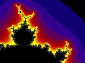
provided enough iterations (n) are done that |z_n| is large. Most fractal artists do not care about electrostatic potential, but they are very interested in continuous values.

Of particular interest to fractal artists who have many images created with the escape-time algorithm is the normalized iteration count algorithm. The primary advantage of this algorithm is that it produces isocontours which are the same as the escape-time algorithm, if given the correct parameters, yet it produces continuous values rather than discrete ones. This direct adaptation can remove the banding from older escape-time images while preserving the rest of the fractal shape. The formula for calculating the normalized iteration count is

An interesting quirk of this formula is that it does not depend on the size of the bailout circle used; for matching up normalized iteration counts with the simpler discrete iteration counts, it is more convenient to use the formula [4]:

                                                                  [4]

where b is the bailout radius.

As a final distance estimator, we introduce e^-|z| smoothing. This simply sums e^-|z| over all iterations; as |z| increases, e^-|z| approaches zero and further iterations change the sum very little. Like normalized iteration counts, as long as the bailout radius is sufficiently large, the precise value bears little impact on the resulting image.

It should be noted that the formulas given above generally apply to the classic z²+c formula. For similar equations where only the exponent is changed, replacing the 2 with the correct exponent is often sufficient. For other fractal equations, more radical reworking may be required. For e^-|z| smoothing, however, no changes are necessary; it works well for almost any divergent series.