|
Vector valued fractal interpolation functions f : R ® R 2 can be introduced in the following setting ( see Barnsley [1], [3], Barnsley et al. [2], Massopust [13], [14]). Given the set of interpolating data D
= {Pi = [xi yi
zi]T Î
R3,
xi
<
xi+1
,
i
= 0, 1,...,
n}, one builds
n affine transformations
wi : R3
®
R3
having the form
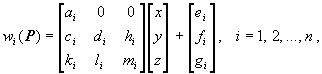
The set s(D) = {R 3; w1, ..., wn} is an affine Iterated Function System (IFS) associated to D. If all the affine mappings wi are contractive, the IFS s(D) is hyperbolic and it has a unique attractor FDÌ R3. This is the fixed point of the Hutchinson operator W( . ) = Èi wi ( . ), a contractive operator on the complete metric space of all non empty compact subsets of R3 endowed with the Hausdorff metric, H(R3, h). Thus, denoting by Wm = W° W m-1, and by G an arbitrary compact subset of R3, the attractor FD satisfies W(FD) = FD, FD = limm ®¥W m( G ). Any sequence of the type
Notice that, despite the uniqueness of the attractor of a hyperbolic IFS, the multitude of its preattractors offers a rich source of of graphically interesting and sometimes aesthetically very pleasent sets. Hutchinson orbits may have various applications, ranging from computer graphics to number theory. Furthermore, the arbitrariness of the initial set G provides extra degrees of freedom which prove useful for modeling purposes. In the interpolation case, given D, the coefficients of transformations wi (i = 1,..., n) can be fixed so that FD is the graph of a continuous vector valued function f : I ® R 2 ( I = [x0 , xn] Ì R ) having the interpolation property, namely a function such that f(xi) = [ yi zi]T (i = 0,1,..., n). This function is called a generalized fractal interpolation function (Barnsley [2], [3]), or simply a vector valued fractal interpolation function (Massopust [13], [14]) and its projections are called hidden variable fractal interpolation functions. For more details see Section 2. A nice application of hidden variable functions is given in Section 3. A shortcoming of the fractal interpolants we deal with is lack of predictability of the shape of their graphs by means of the usual tools of CAGD. The affine invariance of the IFS's whose attractors are graphs of vector valued fractal interpolation functions is examined here, in Section 4. The related results are illustrated by a graphical construction based on visualization of a distance function between prefractal sets. Affine invariance property is one aspect of the problem of predictability and modeling ability of IFS attractors, as dealt with in Kocic and Simoncelli [5]-[11]. Various examples of prefractal sets and applications are also illustrated
here, in Section 5.
|