 |
THE EDUCATIONAL USE OF MATHEMATICAL SOFTWARE:
TECHNIQUES AND EXAMPLES
Aleksandar T. Lipkovski
Faculty of Mathematics, University of Belgrade
ViVe Math - Workshop for visualization and verbalization
of Mathematics and Interdisciplinary Aspects
Niš, December
14-15, 2001
acal@matf.bg.ac.yu
|
Visualisation of mathematical concepts plays a very important role in
mathematical education and research. Needless to say, in addition to standard
visualisation such as drawing graphs, every mathematician has his own internal
visualisation techniques, images which he uses in order to clarify the
mathematics he is thinking of. The visualisation techniques play especially
important role in the process of education. What tools do we have for that
purpose? Until recently, one had to visualise mathematics more or less mentally.
The most important tool, graphing, had its limitations because of objective,
external reasons - human capability of representing clear and nice plots and
drawings. But since the introduction of computers and computer programs designed
for these purposes, graphing techniques became more and more available to ever
wider range of individuals. Computer packages such as Mathematica [7] extended graphing capabilities beyond our imagination of only a decade or two
ago.
In order to
use visualisation as an educational tool, one should be aware of some basic
principles. First, one must have clear understanding of mathematical concepts
which are to be presented. This is, naturally, "conditio sine qua non"
when one starts to think about visualisation. Second, and this is what we shall discuss
here in some detail, is the choice of proper technical
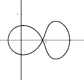
realisation of the task. A simple 2-dimensional drawing of a real function, so
common in the course of calculus provides us with an example on the right,
representing the Serret's plane curve S1/2, arising in
certain connection with the lemniscate (see [1] for details). This curve has
parametric equations
| x=(r6+6r2-2)/r3 |
| y=Ö(r2-x2) |
Even in this simple drawing, we encounter problems with
graphing of implicit functions.
|
 |
 |
But
when we make one step further and draw surfaces in space, or 3-dimensional
objects, we have problems in representing the third dimension,
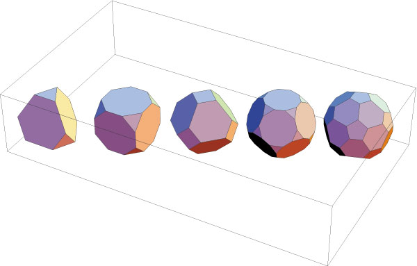
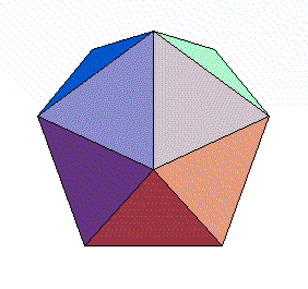
projected to a 2-dimensional drawing plane. Since ancient times,
humans use colour for that purpose, and produce coloured drawings
such as the one on the left, representing the five Platonic solids,
truncated 40%. The role of colour is to represent the effect of
ambient light on 3-dimensional objects. |
However, very often these traditional tools
are not enough. Either the object which we have to represent is too complicated,
or it even does not live in the 3-dimensional, but in some higher dimensional
space. To deal with these two particular problems, we have additional "tips and
tricks".
If a graphical object is to be constructed, one has
several possibilities, depending on its complexity:
| - explicit function drawing
(which has limited scope, as we have seen already in the first graph) |
| - parametrisation, or the use of
parametric representation of functions which we attempt to draw |
| - patching technique, or building the graphical object from separate pieces |
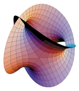 |
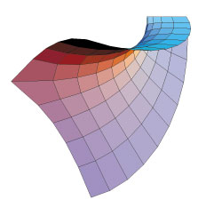
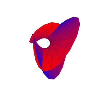
Here, patching technique is demonstrated in
drawing a complex surface with equation
built from 6 individual parametrised patches (right)
(see [5] for details)
|
 |
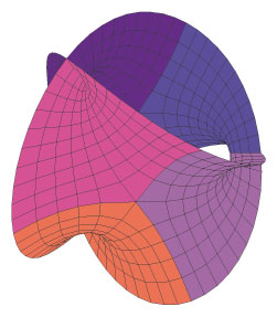
| In addition to
the original ambient light spatial effect, colouring can be used to
represent a complex object or to increase its
artistic appeal. The patch structure of the above surface
can be shown by colour: |
 |
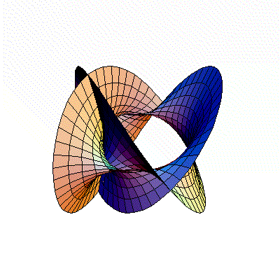
We often need to represent more than 3 dimensions. If we have
2-dimensional surface in 4-dimensional space, we can still use projection R4
® R3, but it may produce
unwanted self-intersections of the surface which does not really exist in 4
dimensions. These self-intersections do show up on the above patch surface.
However, we can use colouring or shading to represent the fourth
coordinate in the projection, as in
[2] (see also below).
In addition to colouring, there is one powerful tool we can
use: motion. It can be used in variety of ways, the most important would be
| - rotational spin shows, and |
| - deformation |
 |
The spin show is useful for looking at the object from
different sides, as this icosahedron on the left demonstrates. The overall look of the above
surface
can be shown also by spin show (right). |
 |
Finally, deformation is certainly an important visualisation
tool, which helps to represent various transformations of mathematical objects.
The reader is invited to have a look at transitions of the topological type of
algebraic curves y2 = x(x-l)(x-m)
when first l ®0 and then m ®
0, demonstrated in [2].
 |
Here we show the appearance of the so-called cusp or
fold, one of the five
Rene
Tom's elementary catastrophes. |
| Here we see the combination of methods
mentioned: colouring represents the fourth coordinate, and deformation and
spin show taken together represent the degeneration of
"alpha" cubic y2 = x2(x-m)
into the "cusp" cubic y2 = x3.
It is a slightly modified version of the animation in [2]: |
 |
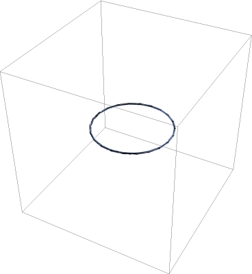
Now, let us have a look at the representation of the interesting Hopf's fibration. If we compactify the 3-space R3
by adding one point ¥ at the infinity, we obtain the
3-sphere S3=R3È{¥}.
Hopf's fibration is the fibration of this 3-sphere into 1-dimensional fibres S1®S3®S2
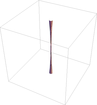 |
It is visualised in this animation. The
circular fibres fill in the whole space, including the point at infinity
(represented by the vertical N-S direction).
On the left, only half of the circular fibres are made visible, in order
to make the interior of the pulsating torus visible too. The clipping is
unavoidable, and occurs at the transparent faces of the surrounding cube. |
 |
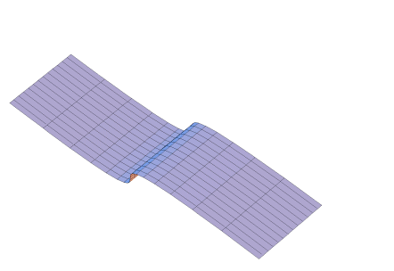
| We will finish this brief overview of simple
methods and examples by showing the deformation of the tensile roof structure in
architecture. The roof is formed by stretching the rubber surface, which
is pinned to the ground at its
corner points, by means of two extending vertical rods. Mathematically,
this reduces to solving the Poisson's second order PDE by finite
differences method and consecutive iteration process (see [4]
for
details): |
 |
Acknowledgements
The author wishes to thank the organizers of the ViVe
workshop, Eberhard Malkowski and Slavik Jablan for the invitation. The idea of the
representation of the surface x3+y2=1
belongs to Hanson [5], and the idea for Hopf's fibration has been communicated
by Jürgen Richter-Gebert, one of the authors of Cinderella [6]. Finally, my thanks are directed
to Wolfram Research Inc for the reviewer's copy of Mathematica 4.1 which has been
used to write the review [3] and to produce the graphical material in this article.
References
[1] A. Lipkovski: Serret's curves. Conference
"Topology and applications", dedicated to P. S. Alexandroff's 100th
birthday, Book of abstracts, Moscow, Phasis, 1996, pp. 191-192
[2] A. Lipkovski: Visualization of simple
algebro-geometric ideas. VisMath, 2:1, 2000, http://www.mi.sanu.ac.yu/vismath/lip
[3] A. Lipkovski: Wolfram's Mathematica
(review in Serbian). Mikro Magazine, March 2001, pp. 43-45
[4] J. Lipkovski: Berechnung und
Formfindung von Membranentragwerken. Seminararbeit, Universität Stuttgart,
2002, http://www.lightstructures.de (under construction)
[5] A.J. Hanson, A construction for computer
visualization of certain complex curves, Notices of the AMS, 41:9, 1994, pp.
1156-1163
[6] J. Richter-Gebert, U.H.
Kortenkamp: Cinderella, the interactive geometry software, Springer-Verlag,
1999, http://www.cinderella.de
[7] S. Wolfram et al: Mathematica Software
Package, version 4.1, Wolfram Research Inc., 2000, http://www.wolfram.com
VisMathHOME