![]()
![]()
![]()
Visual Magic Squares and Group Orbits I
3. Generating
In this section of the
paper we will assume that the reader is familiar with basic finite group theory
at the level of Slomson [7]: Chapter 7.
Permutations and Groups, and Chapter 8. Group Actions. We will continue to pursue the task of
finding all
Definition 3.1. Let (G, •, e) be a group and let X be a non-empty set. Then the group G acts on the set X just in case there is a mapping (a group action) [. , .]: G ´ X → X such that for all g, h in G and x in X: (1) [e, x] = x and (2) [g, [h, x]] = [g • h, x]. Note that in order to simplify notation we will often write g(x) for [g, x].
Base 2 and Base
10 Coding of
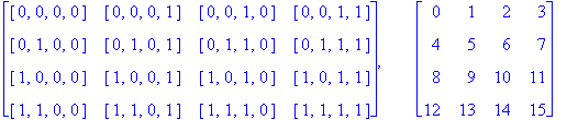
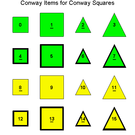
Illustration 3.1
![]()
Definition 3.2. As specified in Definition 2.6, the two main diagonals of
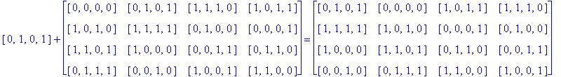
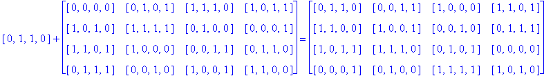
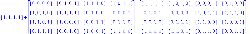
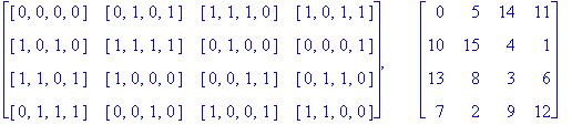
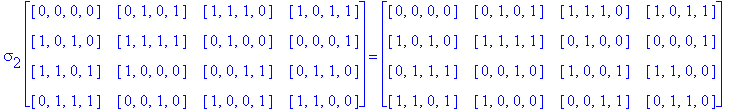
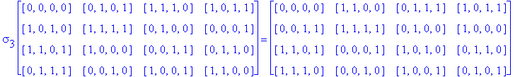
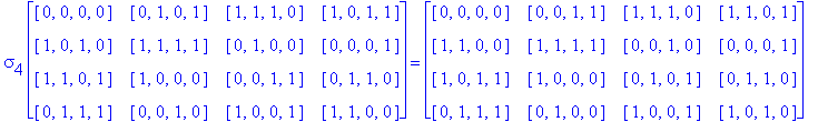
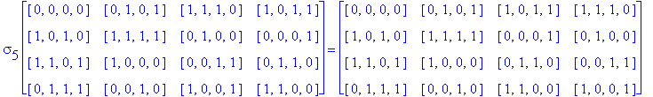
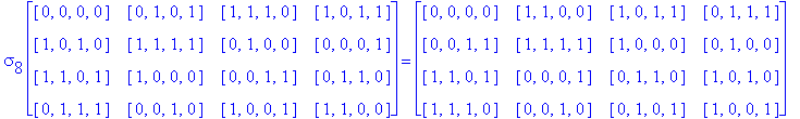
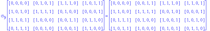
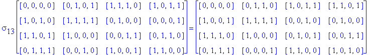
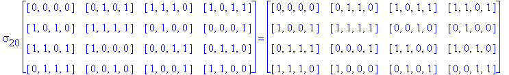
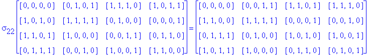
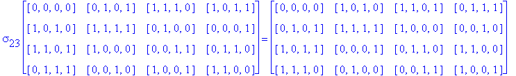
(1) H(4) = {[0, 0, 0, 0], [0, 1, 0, 1], [1, 0, 1, 0], [1, 1, 1, 1], [0, 0, 1, 1], [0, 1, 1, 0], [1, 0, 0, 1], [1, 1, 0, 0]},
(2) K(4) = {[0, 0, 0, 1], [0, 0, 1, 0], [0, 1, 1, 1], [1, 0, 1, 1], [1, 1, 1, 0], [1, 1, 0, 1], [1, 0, 0, 0], [0, 1, 0, 0]},
(3) G(4) = H(4) È K(4).
Then,
G(4) is the set of all
Theorem 3.3.
(1) (G(4), +) is an abelian group isomorphic to C2 ´ C2 ´ C2 ´ C2, where C2 is the cyclic group with two elements.
(2) (H(4), +) is a subgroup of (G(4), +) isomorphic to C2 ´ C2 ´ C2.
(3) For each k in K(4), k + H(4) = K(4), i.e. K(4) is the other coset of (H(4), +) in (G(4), +).
Exercise 3.1. Prove Theorem 3.3.
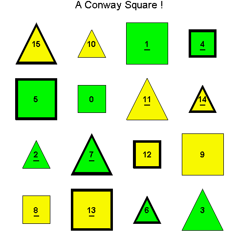
Definition 3.4. Let CS
denote the set of all
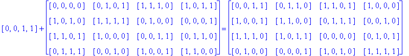
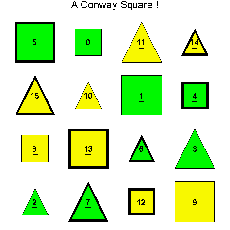
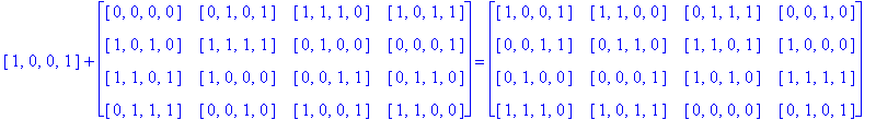
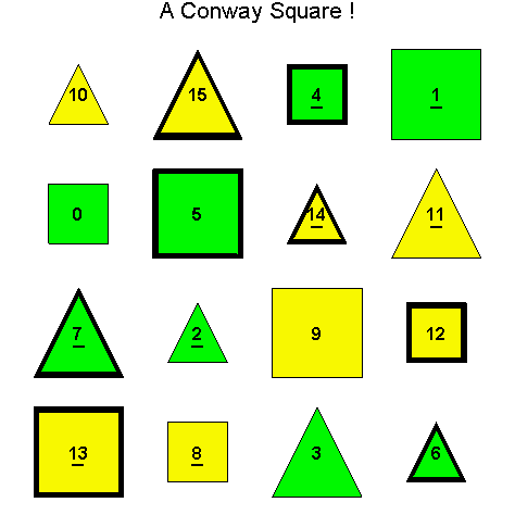
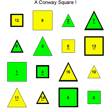
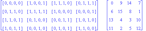
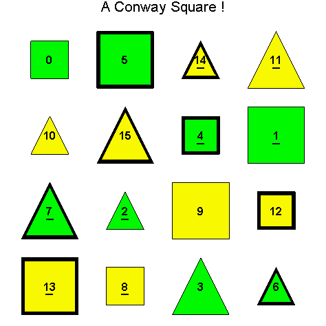
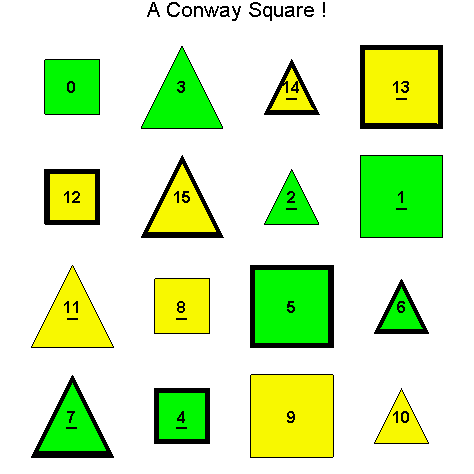
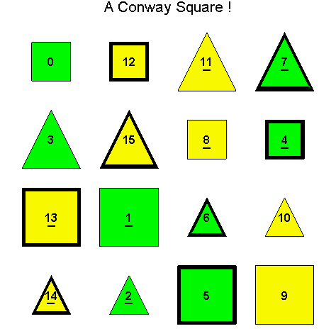
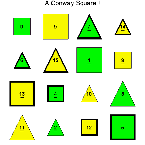
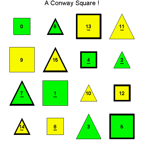
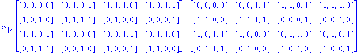
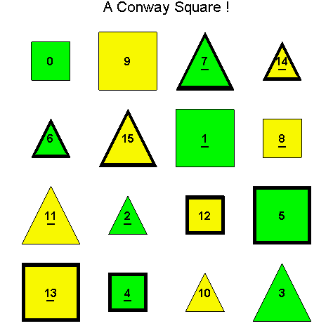
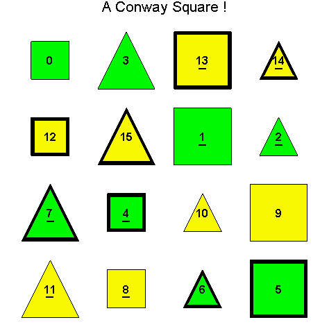
Example 3.5. Let So be the following Type D1 Conway square and consider finding H(4)( So), i.e. the H(4) orbit of the square So.

Base 2 and Base
10 Coding of So ![]()
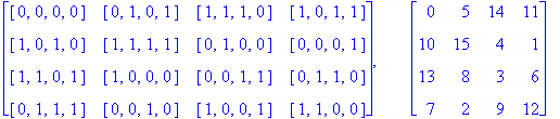
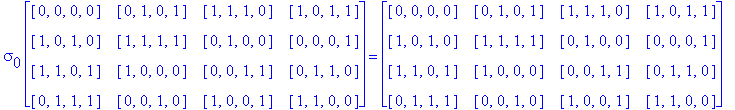
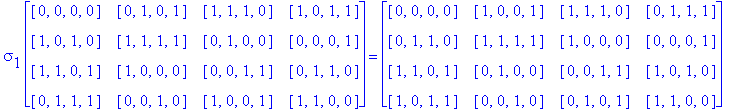
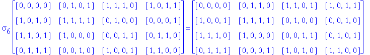
Note that H(4) is easily recognized as the members of G(4) having an even number of 1's. So, to find H(4)( So) we just add each h in H(4) to each entry of So as follows:


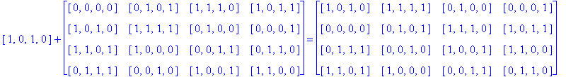


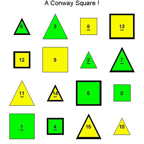
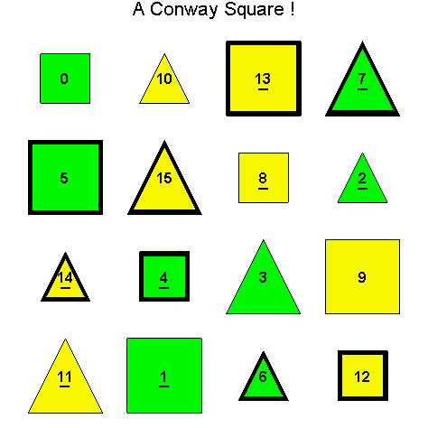
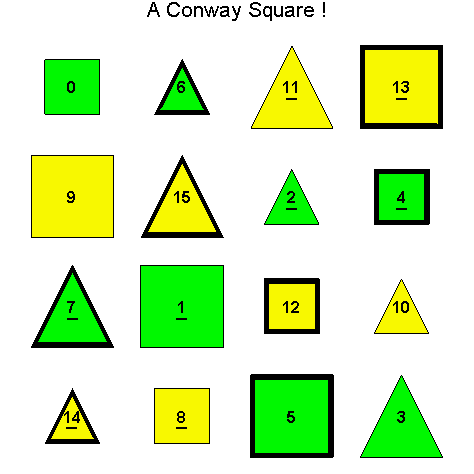
Notice that since So is a Type D1 Conway square, each square h + So is also a Type D1 Conway square:
A Type D1

Another Type D1
![]()
Another Type D1
![]()
Another Type D1

Another Type D1
Another Type D1

Another Type D1
Another Type D1
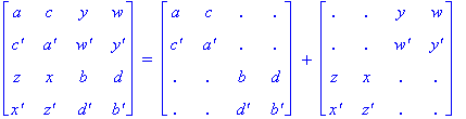
Next, recall from Definition 2.7 that a Type D1 Conway square has the items in the two similarity classes organized as follows:
Notice that in Example 3.5, for each h in H(4) the similarity classes corresponding to H(4) (though scrambled) stayed in the upper left and lower right in h + So, and the similarity classes corresponding to K(4) (though scrambled) stayed in the lower left and upper right in h + So. Furthermore, the pattern of complements above (though scrambled) was preserved for the similarity classes corresponding to both H(4) and K(4) in h + So.
Exercise 3.2. Using the
Motivated by Example 3.5, Exercise 3.2, and our observations above, we have the following theorem.
Theorem 3.6. Let S be a
(1) for all g in G(4), [g , S] = g + S is in CS,
(2) the mapping [ . , S]: G(4) → CS is 1-1,
(3) |G(4)(S)| = |G(4)| = 16,
(4) for all h in H(4), [h , S] = h + S preserves the original location in S of the two similarity classes determined by H(4) and K(4), though scrambling occurs within the locations of both H(4) and K(4).
(5) for all k in K(4), [k , S] = k + S interchanges the original locations in S of the two similarity classes determined by H(4) and K(4).
(6) for all g in G(4), if S is of Type D1, D2, D3, R1, R2, or R3, then [g , S] = g + S is of Type D1, D2, D3, R1, R2, or R3, respectively.
Exercise 3.3. Prove Theorem 3.6.
Definition 3.7. Let D(4) = {Id, Rot90, Rot180, Rot270, FlipH,
FlipV, FlipLD, FlipRD} be the group of symmetries of the geometrical
square (the dihedral group), where the rotations Rot90, Rot180, Rot270
are measured in the clockwise direction, and where FlipH,
FlipV, FlipLD, FlipRD are reflections in the horizontal, vertical, left
main diagonal, right main diagonal axes, respectively. Note that D(4) determines a group action on the set of
In
addition, two
Exercise 3.4.
(1)
Beginning with the same Conway square So as in Example 3.5,
determine how many essentially different Conway squares are in G(4)( So),
i.e. first determine which of these Conway squares are geometrically equivalent
using the group D(4). Note that you may use the following MapleÔ
worksheet [insert link] to help check for essentially different
(2)
Find a subgroup M of G(4) isomorphic to the subgroup {Id, Rot180, FlipH, FlipV} of D(4) such that
the M orbit of So, M(So), contains only Conway squares
geometrically equivalent to So. How do the cosets
of M relate to the essentially different
Remark 3.8. From Theorem 3.6 and Exercise 3.4 we see that the orbit of G(4) on a specific S in CS produces only 16 of the 384 Type D1 Conway squares, and only 4 of the 48 essentially different Type D1 Conway squares (see Theorem 2.8. and Corollary 2.9). Furthermore, it's not hard to see that the same results hold for Type D2 and D3 Conway squares.
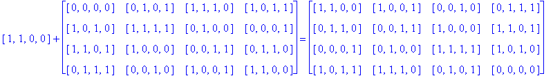
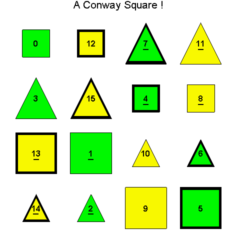
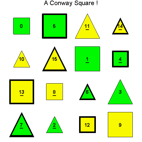
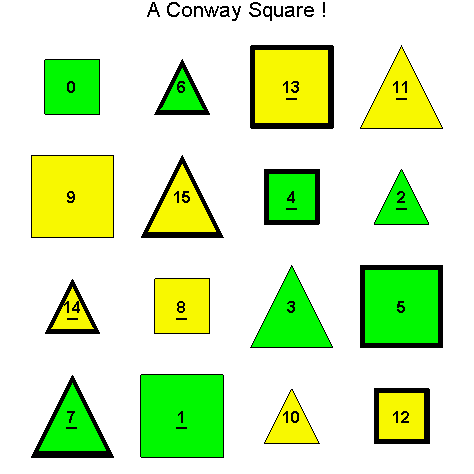
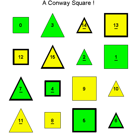
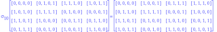
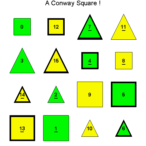
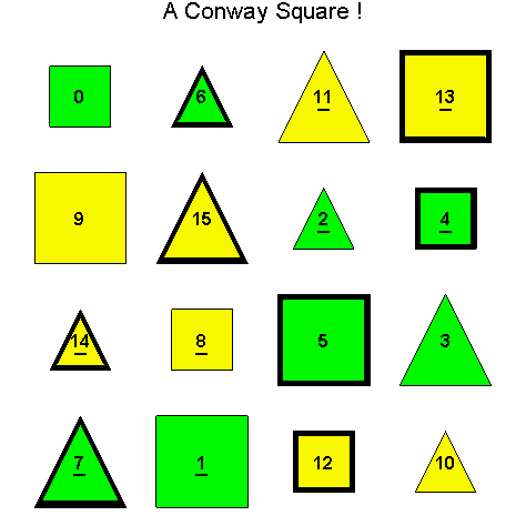
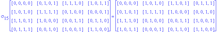
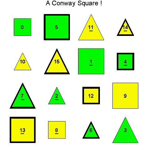
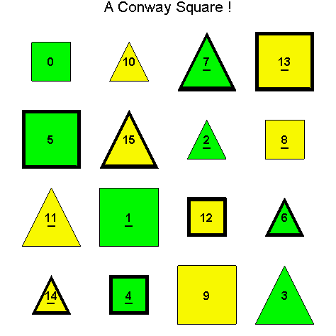
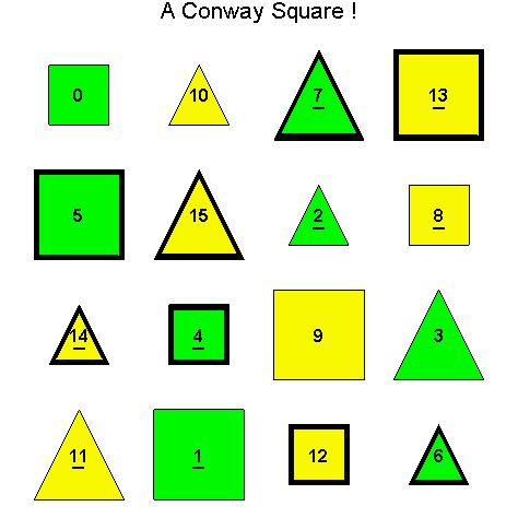
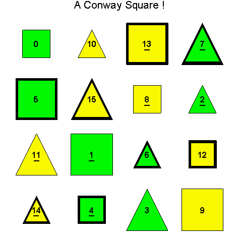
In order to generate still more Type D1 Conway squares, we can again try to find other automorphisms of the group G(4) whose extensions preserve Type D1 Conway squares. Instead of G(4) acting on itself via left translation using the group operation, we can investigate the extension of a simple permutation of the components of g in G(4). For example, let g = [g1, g2, g3, g4] and consider the automorphism [g1, g2, g3, g4] → [g2, g1, g3, g4] which switches the first and second components of g. Let So be the D1 Conway square in Example 3.5, and call the extension of this switch mapping applied to every entry of So, Sw1,2, then Sw1,2(So) is the image of So after switching the first and second components of every entry of So.
Base 2 and Base
10 Coding of So ![]()
Base 2 and Base
10 Coding of Sw1,2( So)
![]()
Notice
that since So was a
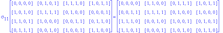
Definition 3.9. In order to define the action of S(4) on CS, we first define the action of S(4) on G(4). Let [. , .]: S(4) ´ G(4) → G(4) be defined by [σ, g] = [gσ(1), gσ(2), gσ(3), gσ(4)] for each σ in S(4) and g = [g1, g2, g3, g4] in G(4). Next, we extend this action to CS. Let [. , .]: S(4) ´ CS → CS be defined by [σ, S] = σ(S), where σ is applied to each entry of S.
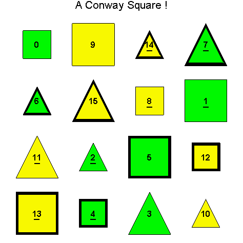
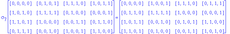
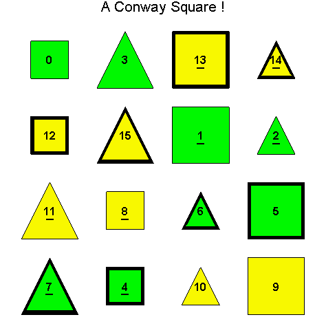
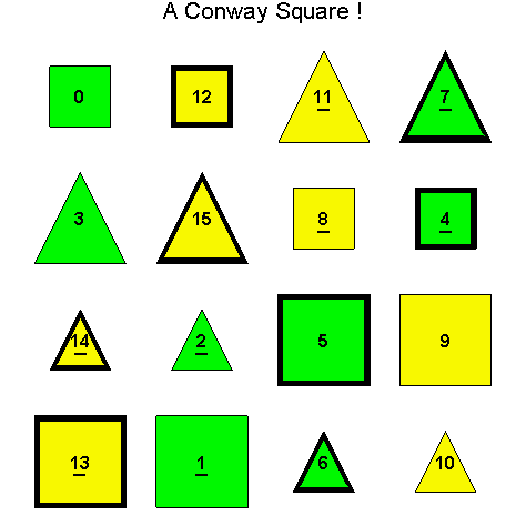
Example 3.10. Once again, we begin with the D1 Conway Square So in Example 3.5. This time we find the S(4) orbit of So.

Another Type D1
![]()
Another Type D1
![]()
Another Type D1
![]()
Another Type D1
![]()
Another Type D1
![]()
Another Type D1
![]()
Another Type D1
![]()
Another Type D1
![]()
Another Type D1
![]()
Another Type D1
![]()
Another Type D1
![]()
Another Type D1
![]()
Another Type D1

![]()
Another Type D1
![]()
Another Type D1
![]()
Another Type D1
![]()
Another Type D1

![]()
Another Type D1
![]()
Another Type D1
![]()
Another Type D1

![]()
Another Type D1
![]()
Another Type D1

![]()
Another Type D1
![]()
Another Type D1
Exercise 3.6. Show that there are only twelve essentially different
Exercise 3.7. Determine the total number of essentially different
Exercise 3.8. Explain why we must have G(4)( So) Ç S(4)( So) = { So } by examining the two different group actions, without using the listings of members of these orbits (above).
Motivated by Example 3.10, and Exercises 3.6-3.8, we have the following theorem.
Theorem 3.11. Let S be a
(1) for all σ in S(4), [σ, S] = σ(S) is in CS,
(2) the mapping [. , S]: S(4) → CS is 1-1,
(3) |S(4)(S)| = |S(4)| = 24,
(4) for all σ in S(4), σ(S) preserves the original location in S of the two similarity classes determined by H(4) and K(4), though scrambling occurs within the locations of both H(4) and K(4).
(5) for all σ in S(4), if S is of Type D1, D2, D3, R1, R2, or R3, then σ(S) is of Type D1, D2, D3, R1, R2, or R3, respectively.
Exercise 3.9. Prove Theorem 3.11.
Remark 3.12. We have shown that if S is a Conway square in CS then |G(4)(S)| = 16 and |S(4)(S)| = 24, but these still fall far short of the totals for each type found in Theorems 2.8 and 2.12, e.g. there are 384 Type D1 Conway squares. However, it is natural to think about combining these two group actions. For example, suppose for each sigma in S(4), we consider the orbit of G(4) on sigma(S), i.e. for each g in G(4) consider g + sigma(S). Note that we have already done this in the case that sigma = Id, which is just the orbit of G(4) on S. This approach is particularly encouraging, since |G(4)(S)| |S(4)(S)| = (16)(24) = 384.
Definition 3.13. We now define the
Note that as usual B(4) acts on itself, but we want to restrict this action to G(4), in order to then extend it to the set of all Conway squares CS. First, we define the restricted action of B(4) on G(4) by [(g, σ), (h, Id)] = (g, σ) • (h , Id) = (g + σ(h), h), where we simplify notation and simply write [(g, σ), h] = g + σ(h). Next, we define the action of B(4) on CS by [(g, σ), S] = g + σ(S).
Exercise 3.10. Verify that (B(4), •) is a group.
Theorem 3.14. (Conway Group Orbit Theorem)
Let
S be a
(1) for all σ in B(4), [(g, σ), S] = g + σ(S) is in CS,
(2) the mapping [. , S]: B(4) → CS is 1-1,
(3) |B(4)(S)| = |B(4)| = 384,
(4) for all (g, σ) in B(4), if S is of Type D1, D2, D3, R1, R2, or R3, then g + σ(S) is of Type D1, D2, D3, R1, R2, or R3, respectively.
Corollary 3.15. The action of the
Exercise 3.11. Prove Theorem 3.14.
Exercise 3.12. Verify Corollary 3.15 using the Euler squares you found in Exercises 1.2 and 1.3 as the seeds to generate the seven B(4) orbits, and the following MapleÔ worksheet [insert link].
Exercise 3.13. Repeat Exercise 3.14 using the Conway squares provided as examples in the proofs of Theorems 2.8 and 2.12, as the seeds to generate the seven B(4) orbits, and the following MapleÔ worksheet [insert link].
Exercise 3.14. Examine each of the orbits of B(4) in Exercise 3.12 and
determine which elements of B(4) form a subgroup isomorphic to (a subgroup of) D(4)
that determines the geometrically equivalent
Exercise 3.15. Using your results in Exercise 3.14 verify the number of essentially different Conway squares of each type found in Corollaries 2.9 and 2.13. Here is a helpful MapleÔ worksheet [insert link].
Exercise 3.16. (Generating Euler Squares I) We know
that there are Euler squares of each of the six different types of
Exercise 3.17. (Generating Euler Squares II) Repeat
Exercise 3.16, using the same hint, but let F be the group (S(4) ´ S(4), ο), instead of
(Z4 ´ Z4, +). Once again, let E(2) = F ´ S(2), with group operation defined as in B(4), and find
the orbit of E(2), restricted to F, on the smallest set of Euler squares needed
to generate them all.
Remark 3.15. In a sequel to this paper [5], we extend
this approach to the remaining (352) NonConway 4 ´ 4 magic squares, developing additional types and using
appropriate group orbits to generate them all. In addition, we explore the extension of these ideas to the
analysis of higher order magic squares.
![]()
![]()
![]()