|
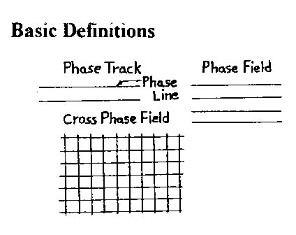
Basic Definitions
Figure 2.1
Figure 2.2
Figure 2.3 Refer to Fig. 2.1 for the following definitions. Phase
Line: a continuous line division of space.
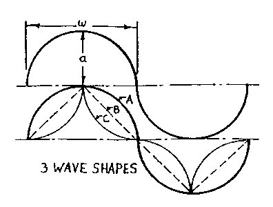
Cross Phase Field: the crossing of two or more phase fields. Wave dimensions and wave shapes are seen in Fig. 2.2 where w is 1/2 the basic wavelength W, and a is its amplitude - the three basic wave shapes assumed are the common wave A, the line wave B, and the concave wave C. Common Wave Space (CWS) is defined by a curvilinear coordinate system. It is a wave gnid pattern formed using an X or Y phase field orientation with one field a function of the other. This is what I call a functional geometric system and should not be confused with an overlay system where one phase field is randomly overlaid on another. Interphase Wave Space (IWS) is a wave pattern formed by plotting a second generation wave field on a CWS grid. Wave
Space Equation
where each
term is drawn sequentially, Y1 and X1
indicate the primary wave field directions, the X1 field
being a function of the Y1 field to form a CWS grid configuration.
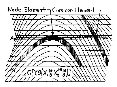
X2 is the secondary wave field taken as a function of, and interphasing
with the CWS coordinate grid. Interphasing occurs when one field track
intercepts another, going in the same direction, and returns without
crossing. The shape formed, I call a nodal
element, or node en. The other elemental shape
which is formed by two or more phase tracks crossing
each other, I call a common element ec,
as seen in Fig. 2.3. CWS is made of totally common elements;
IWS is the summation of common and nodal elements in a proportion dependent
on the interphasing geometries.
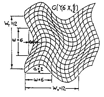
Figure 2.4 Common Wave Space (CWS)
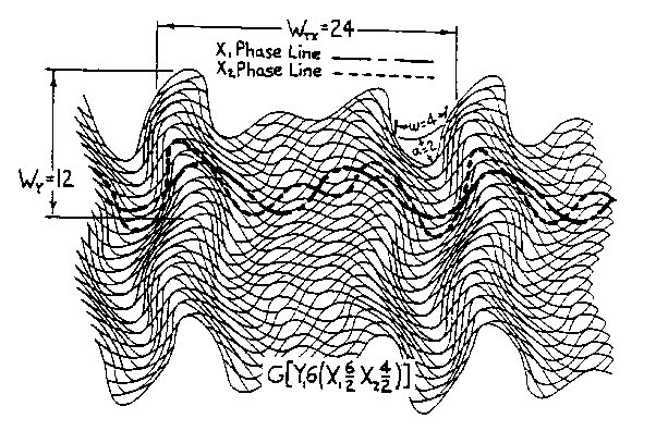
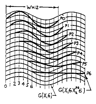
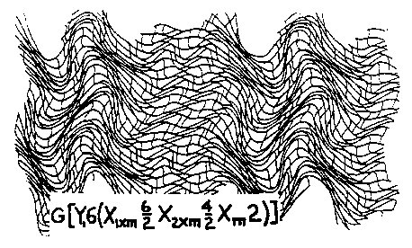
Figure 2.5 Interphase Wave Space (IWS) An example of CWS is seen in Fig.2.4 where wY1=6, aY1=1, and wX1=6, aX1=2, or SW=G(Y16/1X16/2), written G(Y16X16/2). An example of IWS is seen in Fig. 2.5 where the X2 field of wX2=4, aX2=2 interphases with the CWS coordinate system of Fig. 2.4 in the X1 direction, the third term of Sw, The pq superscript in Sw indicates the phase position of the secondary wave on the primary wave and determines the rhythm of the interphase field as shown in Fig. 2.6.There are W possible starting positions on wavelength W; in our example, 7 out of 12 positions are shown in aG(X16) wave field interacting with a secondary X26 wave field. In Fig. 2.4 there are also 12 possible positions:W=2wX1=2×6=12. In example, Fig. 2.5, q=0 was chosen to establish the secondary X24/2 interphase wave field.Also note in the equation G[Y16(X16/2X24/2)] of Fig. 2.5 that the parenthetic bracketing indicates what is shown, and will be so in subsequent equations.
Figure 2.6 Phase Positions
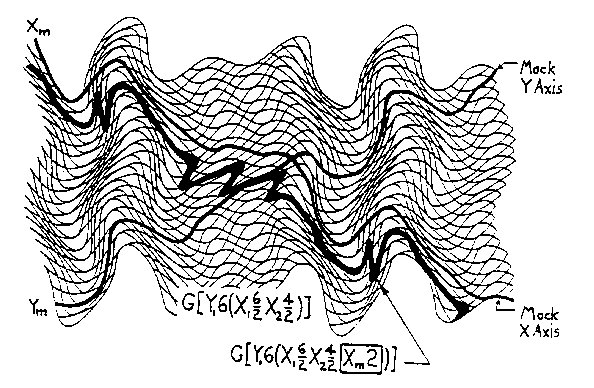
Figure 2.7 Mock Axes The fourth
term of Sw, is what I call a mock
axes coordinate system; in other words, a IWS configuration used
as CWS grid. This is done by choosing an axes intersection point, i.e.,
an origin, with one coordinate starting in the primary field direction,
the other starting in the secondary field direction and at each node alternating
to the other field direction, giving the continuous, divergent x,y
mock axes Xm and Ym as exemplified
in Fig. 2.7. (Notice Xm is drawn from
the upper left to lower right and Ym from the lower left
to upper right). The "layered" position of Xm and Ym
of SW, means that an Xm interphase
field, orYm interphase field,
or
both simultaneously can be plotted. Fig.2.7 shows the
single interphase track Xm2.
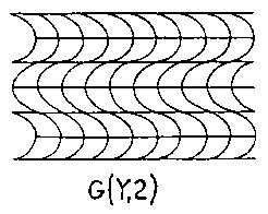
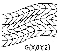
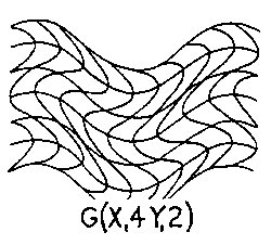
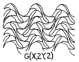
Figure 2.8 CWS
Figure 2.9 CWS
Figure 2.10 CWS
Figure 2.11 CWS The above examples are given to further demonstrate how Wave Space works. CWS Figs. 2.8, 2.9, 2.10, 2.11 show a progression in wave dynamics holding aX1, and Y12 constant with wX1, going from infinity to 2. Isolating
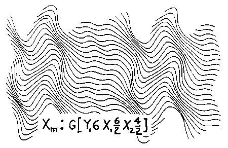
the mock axis field
Xm of Fig. 2.5,
we have Fig. 2.12. The semi-colon in equations such
as Xm: G(...) and Ym: G(...)
simply means Xm or Ym of the specific
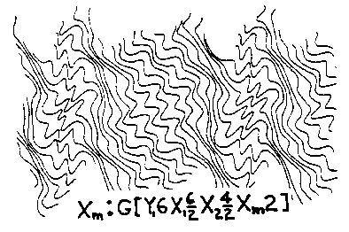
geometry G(...). Fig. 2.13 is an extension ofFig.
2.5 space in the mock
X axis direction by
Xm2.
Figure 2.12 IWS
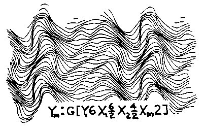
Figure 2.13 IWS Figs. 2.14 and 2.15 is Fig. 2.13 separated into its Xm and Ym phase fields. Fig. 2.16 is formed by extending Fig. 2.5 in both mock axes directions simultaneously.
Figure 2.14 IWS
Figure 2.15 IWS 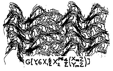
Figure 2.16 IWS Variation is further increased if we consider the shape of the wave w, or wave-train WT. Wave shape A was used in the previous examples. The other two basic shapes B and C, Fig. 2.3, should be noted. Figs. 2.17 and 2.18 show the B and C waves in the Fig. 2.4 CWS geometry; Figs. 2.19 and 2.20 show the B and C waves in the Fig. 2.5 IWS geometry. The symbol above the wave dimensions indicates the wave type and its orientation: ~ indicates a full wave; Ç È indicates a half wave oriented apex up or down respectively. 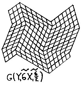
Figure 2.17 CWS B Wave 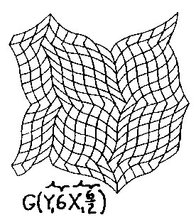
Figure 2.18 CWS C Wave 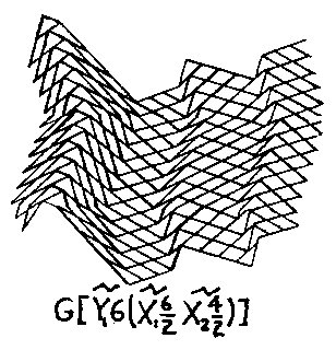
Figure 2.19 IWS B Wave 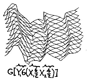
Figure 2.20 IWS C Wave Another approach is the compounding of wavelengths and/or wave shapes as seen in Figs. 2.21 and 2.22 in CWS, with a more complex CWS version in Fig. 2.23 and its IWS extension, Fig. 2.24. The various squiggles, as usedabove, show the specific make-up of a wave shape or wave train. 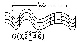
Figure 2.21 CWS Compound Length 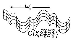
Figure 2.22 CWS Compound Shape 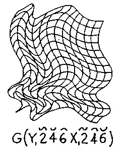
Figure 2.23 Compound CWS 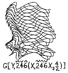
Figure 2.24 Compound M7S
|