| |
|
|
|
|
|
| [BACK: Introduction] |
[NEXT: Case
Study of Aesthetic Forms] |
One of the major purposes of this study is to seek new forms, which is obtained from recording the trajectories of relative motions. For the convenience of further discussion, the concepts required to achieve this are introduced below.
There are many different kinds of motions that exist in real life, such as linear motion, circular motion, simple harmonic motion and spiral motion, etc. There are also numerous motions that do not exist in the real world, such as an object moving in hexagon. Since we are working in the world of computer, where the physical rules of gravity does not apply, we paid equal attention to both kinds of motions.
In order to visualize each kind of motions individually, it is necessary to simulate the motions separately in the beginning. We are used to conceptualize motions and forms on still coordinate systems. The trajectories are difficult to predict if the motion is based on a dynamic coordinate system, that is, the coordinate system itself is also in certain kind of motion.
The factors influencing the trajectories of relative motions include: a. The motion of the point. |
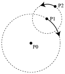 Figure 2-1 |
There are infinite points on any given surface in strict mathematical sense. However, for the purpose of calculation, we assumed that a plane is composed of points that are countable. Each point, the smallest unit of the motion, is measured by pixel. Hence, there are exactly 307,200 pixels on a computer screen of 640 x 480; and the center of the screen is represented by point (320, 240). Moreover, the origin is set on the lower-left corner of the screen instead of the center for the sake of programming.
| Each trajectory in this study is obtained from tremendous amount of iterations (in an average of 10,000,000). How to record the results thus became a problem to solve in the early stages. We used 640 arrays to represent each of the columns of the computer screen, with 480 values in each of the arrays (Figure 2-2). All 307,200 values are set to be zero in the beginning, and the values increase according to the frequencies of visits of the motions (Figure 2-3). We were able to keep record of the movements in this way. And the values, when retrieved and assigned appropriate colors, are used to unfurl the images hidden. | 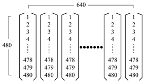 Figure 2-2 |
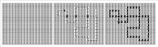
Figure 2-3
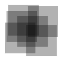
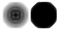
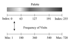
We used only gray-scale images for our pilot study. The color of moving point is set to be black, but with only 30 percent of opacity (in other words, 70 percent transparent). The background is white. Each visit on an identical point will increase the opacity of it (in other words, make it darker by 30 percent). As a result, the more visits a certain point receives, the darker it appears, as shown in Figure 2-4. Interesting shapes did emerge in this way. The problem, though, is that everything tended to fade away when the number of iterations became considerably large (over a million, for instance). Every image ended up with a black mass (usually in the shape of a donut) without any satisfactory details, as shown in Figure 2-5. These donuts made us realize that recording the frequencies of point visits (as introduced above) is critical. In order to assign different colors to the values stored in the arrays, we first divided the values into n levels (e.g., n = 256). The minimum and maximum values in the arrays are then assigned 0 and 255 respectively, which in an 8-bit color palette depict the colors white and black. That is, a pixel on the screen is set to be white if it receives the least visits, or black if it receives the most. The rest 254 levels are assigned different colors according to the color palette, so that different frequencies of visits can be represented with different colors (Figure 2-6). The similarity of colors is determined by how close the levels are, so as to simulate the gradient. Therefore, adjacent levels of frequencies, such as 134 and 135, are assigned similar colors; while levels 25 and 193 are assigned colors that are distinctly different (Figure 2-7). We have to admit that the design of the color palette (e.g., to determine the 254 individual colors) is somewhat arbitrary. There seemed no way for us to determine whether it was the "best" palette for an image, because the judgement was usually quite subjective. As a result of this unsolved problem, the colors of the images in this study may not be the most appropriate ones in the aesthetic sense (Figure 2-8). |
|
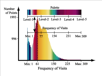 Figure 2-7 |
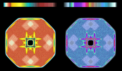 Figure 2-8 |
The trajectories shapes are determined primarily by the relative velocity and magnitude between the moving point and the coordinate system. Findings from earlier studies (Sun, 1999) suggest that the trajectories are sensitive to the initial conditions of the motions. Slight variations of the parameters may end up with shapes that are significantly different. As a result, it is highly difficult to predict how the shapes may look like before they are finished. Obviously, the possibilities can never be exhausted. However, efforts have been made to "systematically" manipulate the parameters in order to explore as many possibilities as possible.
Sun (1999) experimented on iteration of dynamic multiple-level relative motions. He assumed that the sun serves as the origin of an absolute coordinate system, which does not move; and the orbits of both the earth and the moon fall on a same plane. The earth orbits the sun clockwise, and the moon orbits the earth counterclockwise. The trajectory of the moon is more interesting than that of the earth, primarily because the motion of the moon is relative. The trajectory of motions looks like petals. If we manipulate the different relationship of the relative velocities of the earth and the moon, the different results depicted in Figure 2-9. The trajectories in Figure are movements of the moon.
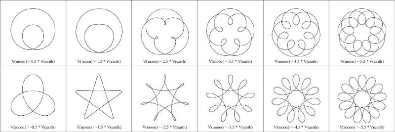
Figure 2-9
In order to make things even more complicated; he added a space ship to orbit the moon counterclockwise, an astronaut to orbit the space ship clockwise, and finally a Mighty Mouse to orbit the astronaut counterclockwise. Each trajectory of the motions depicts the second, the third, and the fourth level of relative motions respectively. The trajectories of each dynamic multiple-level motion system appear rather interesting. The different results of relative motions are shown in Figure 2-10.
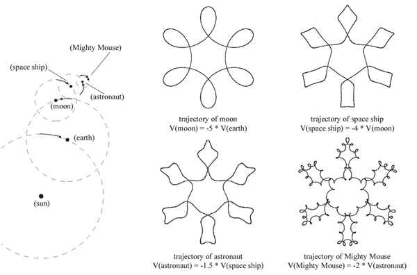
Figure 2-10
The concept of chaotic relative motions is somewhat difficult to explain, primarily because these kinds of motions do not exist in real world. Taking the solar system as an example: the earth orbits the sun, and the moon orbits the earth. The trajectory of the earth is a circle (proximately), and the trajectory of the moon has the shape of petals.
Since the mass of the earth is much greater than that of the moon, it seems that the earth is much more dominant than the moon in terms of their trajectories. That is, the earth almost solely determines the motion of the moon. But the moon, on the other hand, has very little influence on the motion of the earth.
Assuming that the moon can also influence the motion of the earth in a certain way, then the moon is no longer so obedient. That is, the motion of the earth determines the motion of the moon, and the latter determines the former simultaneously. The output of each calculation then becomes the input of itself. This recursive nature would make the motions highly chaotic, resulting trajectories beyond our imaginations.
|
The term pursuit curve in many mathematical books simply considers a chaser in pursuit of a target. It is also called pursuit problem what means an object or target moves along a given curve and a second object or pursuer follows or pursues the target. The object move in the direction of the target at all times (Erwin, 1988). For instance, an airplane moves along the axis with constant speed (Figure 2-11). Find the path of the missile which moves the left-hand of the xy plane with constant speed and always points directly at the target (Sokolnikoff, 1967). Imagine a rabbit and a pizza moving in circles with radii R-rabbit and R-pizza in different speeds. A dog, who is fond of both, is chasing them. Assume that the dog only chases the one that is closer, and it changes its target whenever the other becomes closer. It would be interesting to see how the trajectory of the dog may turn out to be. The trajectories of pursuit motions can be highly complicated. When the systems of multi-level relative motions increased, the trajectories became unpredictable and sometimes peculiar. We experimented two kinds of rules in pursuit relative motions: (1) always pursue the nearest coordinate system, and (2) always pursue the farthest coordinate system. Trajectories of these two kinds of pursuit relative motions appear quite different. |
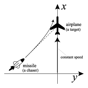 Figure 2-11 |
The process in this study was not only painstaking but also extremely time consuming. It was necessary to develop a proper applet (as shown in Figure 2-12) to take over the routine jobs. The functions of this applet include:
|
|
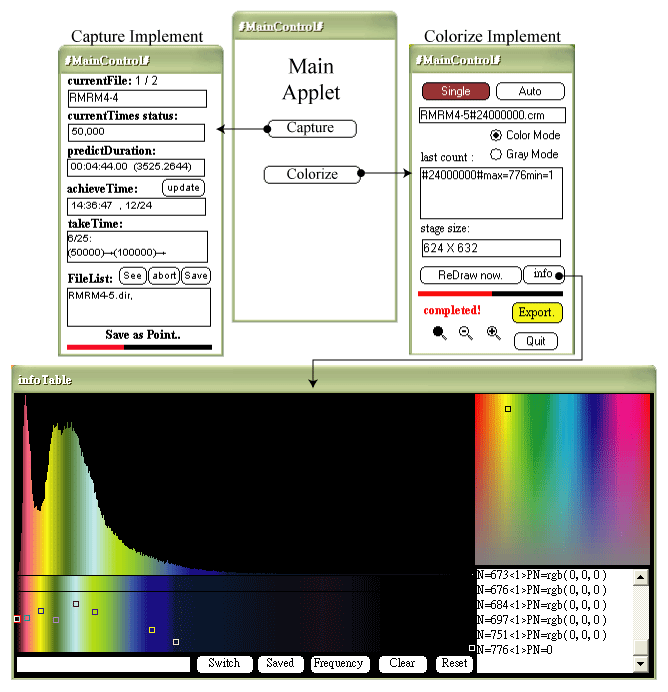
Figure 2-12
|
[BACK: Introduction] |
[NEXT: Case
Study of Aesthetic Forms] |
CONTENTS:
| Conclusions |